AbsorptionModel Tutorial
Trey V. Wenger (c) July 2025
Here we demonstrate the basic features of the AbsorptionModel model. AbsorptionModel models 21-cm 1-exp(-optical depth) spectra like those obtained from typical HI absorption observations. Please review the bayes_spec documentation and tutorials for a more thorough description of the steps outlined in this tutorial: https://bayes-spec.readthedocs.io/en/stable/index.html
[1]:
# General imports
import time

import matplotlib.pyplot as plt
import arviz as az
import pandas as pd
import numpy as np
import pymc as pm

print("pymc version:", pm.__version__)
print("arviz version:", az.__version__)

import bayes_spec
print("bayes_spec version:", bayes_spec.__version__)

import caribou_hi
print("caribou_hi version:", caribou_hi.__version__)

# Notebook configuration
pd.options.display.max_rows = None
pymc version: 5.22.0
arviz version: 0.22.0dev
bayes_spec version: 1.9.0
caribou_hi version: 4.1.0+3.g94a913e.dirty
Simulating Data
To test the model, we must simulate some data. We can do this with AbsorptionModel, but we must pack a “dummy” data structure first. The model expects the observation to be named "absorption".
[2]:
from bayes_spec import SpecData
# spectral axes definition
velo_axis = np.linspace(-50.0, 50.0, 200) # km s-1
# data noise can either be a scalar (assumed constant noise across the spectrum)
# or an array of the same length as the data
rms = 0.001 # 1 - exp(-tau)
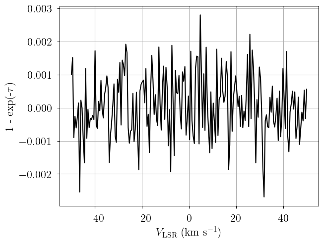
# brightness data. In this case, we just throw in some random data for now
# since we are only doing this in order to simulate some actual data.
absorption = rms * np.random.randn(len(velo_axis))
dummy_data = {"absorption": SpecData(
velo_axis,
absorption,
rms,
xlabel=r"$V_{\rm LSR}$ (km s$^{-1}$)",
ylabel=r"1 - exp(-$\tau$)",
)}
# Plot dummy data
fig, ax = plt.subplots(layout="constrained")
ax.plot(dummy_data["absorption"].spectral, dummy_data["absorption"].brightness, "k-")
ax.set_xlabel(dummy_data["absorption"].xlabel)
_ = ax.set_ylabel(dummy_data["absorption"].ylabel)
Now that we have a dummy data format, we can generate a simulated observation by evaluating the model. First we create the model.
[3]:
from caribou_hi import AbsorptionModel

# Initialize and define the model
n_clouds = 3
baseline_degree = 0
model = AbsorptionModel(
    dummy_data,
    n_clouds=n_clouds,
    baseline_degree=baseline_degree,
    seed=1234,
    verbose=True
)
model.add_priors(
    prior_tau_total=1.0, # total optical depth prior width (km s-1)
    prior_tkin_factor=[2.0, 2.0], # kinetic temperature prior shape
    prior_fwhm2=200.0, # FWHM^2 prior width (km2 s-2)
    prior_log10_nHI=[0.0, 1.5],  # log10(density) prior mean and width (cm-3)
    prior_velocity=[-15.0, 15.0],  # lower and upper limit of velocity prior (km/s)
    prior_log10_n_alpha=[-6.0, 1.0],  # log10(n_alpha) prior width (cm-3)
    prior_fwhm_L=None,  # Assume Gaussian line profile
    prior_baseline_coeffs=None,  # Default baseline priors
)
model.add_likelihood()
Now we simulate with a given set of simulation parameters.
[4]:
from caribou_hi import physics
# Simulation parameters
log10_nHI = np.array([1.25, 0.0, -0.5])
tkin = np.array([50.0, 300.0, 5000.0])
log10_n_alpha = np.array([-5.5, -6.0, -6.5])
depth = np.array([5.0, 25.0, 300.0])
nth_fwhm_1pc = np.array([1.25, 1.75, 1.5])
depth_nth_fwhm_power = np.array([0.2, 0.3, 0.4])
tspin = physics.calc_spin_temp(tkin, 10.0**log10_nHI, 10.0**log10_n_alpha).eval()
print("tspin", tspin)
fwhm_nonthermal = physics.calc_nonthermal_fwhm(depth, nth_fwhm_1pc, depth_nth_fwhm_power)
fwhm2_thermal = physics.calc_thermal_fwhm2(tkin)
fwhm = np.sqrt(fwhm_nonthermal**2.0 + fwhm2_thermal)
print("fwhm", fwhm)
tkin_max = physics.calc_kinetic_temp(fwhm**2.0)
tkin_factor = tkin / tkin_max
print("tkin_factor", tkin_factor)
log10_Pth = np.log10(tkin) + log10_nHI
print("log10_Pth", log10_Pth)
log10_NHI = log10_nHI + np.log10(depth) + 18.489351
print("log10_NHI", log10_NHI)
tau_total = physics.calc_tau_total(10.0**log10_NHI, tspin)
print("tau_total", tau_total)
sim_params = {
"tau_total": tau_total,
"tkin": tkin,
"tkin_factor": tkin_factor,
"fwhm2": fwhm**2.0,
"log10_nHI": log10_nHI,
"velocity": np.array([-5.0, 5.0, 10.0]),
"log10_n_alpha": log10_n_alpha,
"baseline_absorption_norm": [0.0],
}
# add derived quantities to sim_params
for key in model.cloud_deterministics:
if key not in sim_params.keys():
sim_params[key] = model.model[key].eval(sim_params, on_unused_input="ignore")
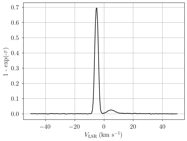
# Evaluate and save simulated observation
absorption = model.model["absorption"].eval(sim_params, on_unused_input="ignore")
data = {"absorption": SpecData(
velo_axis,
absorption,
rms,
xlabel=r"$V_{\rm LSR}$ (km s$^{-1}$)",
ylabel=r"1 - exp(-$\tau$)",
)}
tspin [  49.9920589   297.73994712 2795.52422645]
fwhm [ 2.29393108  5.90364916 21.08270953]
tkin_factor [0.43474124 0.3938236  0.5146817 ]
log10_Pth [2.94897    2.47712125 3.19897   ]
log10_NHI [20.438321   19.88729101 20.46647225]
tau_total [3.01140471 0.14216839 0.05745901]
[5]:
sim_params
[5]:
{'tau_total': array([3.01140471, 0.14216839, 0.05745901]),
 'tkin': array([  50.,  300., 5000.]),
 'tkin_factor': array([0.43474124, 0.3938236 , 0.5146817 ]),
 'fwhm2': array([  5.26211978,  34.85307344, 444.48064099]),
 'log10_nHI': array([ 1.25,  0.  , -0.5 ]),
 'velocity': array([-5.,  5., 10.]),
 'log10_n_alpha': array([-5.5, -6. , -6.5]),
 'baseline_absorption_norm': [0.0],
 'tspin': array([  49.9920589 ,  297.73994712, 2795.52422645]),
 'log10_Pth': array([2.94897   , 2.47712125, 3.19897   ]),
 'log10_NHI': array([20.438321  , 19.88729101, 20.46647225]),
 'log10_depth': array([0.69897   , 1.39794001, 2.47712125])}
[6]:
# Plot data
fig, ax = plt.subplots(layout="constrained")
ax.plot(data["absorption"].spectral, data["absorption"].brightness, "k-")
ax.set_xlabel(data["absorption"].xlabel)
_ = ax.set_ylabel(data["absorption"].ylabel)
Model Definition
Finally, with our model definition and (simulated) data in hand, we can explore the capabilities of AbsorptionModel.
[7]:
# Initialize and define the model
n_clouds = 3
model = AbsorptionModel(
    data,
    n_clouds=n_clouds,
    baseline_degree=baseline_degree,
    seed=1234,
    verbose=True
)
model.add_priors(
    prior_tau_total=1.0, # total optical depth prior width (km s-1)
    prior_tkin_factor=[2.0, 2.0], # kinetic temperature prior shape
    prior_fwhm2=200.0, # FWHM^2 prior width (km2 s-2)
    prior_log10_nHI=[0.0, 1.5],  # log10(density) prior mean and width (cm-3)
    prior_velocity=[-15.0, 15.0],  # lower and upper limit of velocity prior (km/s)
    prior_log10_n_alpha=[-6.0, 1.0],  # log10(n_alpha) prior width (cm-3)
    prior_fwhm_L=None,  # Assume Gaussian line profile
    prior_baseline_coeffs=None,  # Default baseline priors
)
model.add_likelihood()
[8]:
# Plot model graph
model.graph().render('absorption_model', format='png')
model.graph()
[8]:

[9]:
# model string representation
print(model.model.str_repr())
baseline_absorption_norm ~ Normal(0, 1)
              fwhm2_norm ~ Gamma(0.5, f())
          log10_nHI_norm ~ Normal(0, 1)
           velocity_norm ~ Beta(2, 2)
      log10_n_alpha_norm ~ Normal(0, 1)
          tau_total_norm ~ HalfNormal(0, 1)
             tkin_factor ~ Beta(2, 2)
                   fwhm2 ~ Deterministic(f(fwhm2_norm))
               log10_nHI ~ Deterministic(f(log10_nHI_norm))
                velocity ~ Deterministic(f(velocity_norm))
           log10_n_alpha ~ Deterministic(f(log10_n_alpha_norm))
               tau_total ~ Deterministic(f(tau_total_norm))
                    tkin ~ Deterministic(f(tkin_factor, fwhm2_norm))
                   tspin ~ Deterministic(f(tkin_factor, log10_n_alpha_norm, fwhm2_norm, log10_nHI_norm))
               log10_Pth ~ Deterministic(f(log10_nHI_norm, tkin_factor, fwhm2_norm))
               log10_NHI ~ Deterministic(f(tau_total_norm, tkin_factor, log10_n_alpha_norm, fwhm2_norm, log10_nHI_norm))
             log10_depth ~ Deterministic(f(log10_nHI_norm, tau_total_norm, tkin_factor, log10_n_alpha_norm, fwhm2_norm))
              absorption ~ Normal(f(tau_total_norm, baseline_absorption_norm, velocity_norm, fwhm2_norm), <constant>)
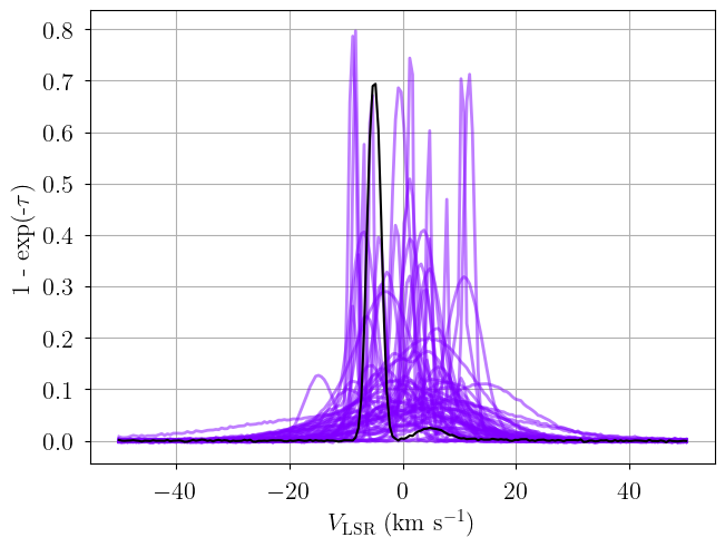
We check that our prior distributions are reasonable by drawing prior predictive checks. Each colored line is a simulated “observation” with parameters drawn from the prior distributions. You should check that these simulated observations at least somewhat overlap your actual observation (black line).
[10]:
from bayes_spec.plots import plot_predictive

# prior predictive check
prior = model.sample_prior_predictive(
    samples=1000,  # prior predictive samples
)
_ = plot_predictive(model.data, prior.prior_predictive.sel(draw=slice(None, None, 20)))
Sampling: [absorption, baseline_absorption_norm, fwhm2_norm, log10_nHI_norm, log10_n_alpha_norm, tau_total_norm, tkin_factor, velocity_norm]
We can also check out our prior distributions impact the deterministic (derived) quantities in our model. The red points represent the simulation parameters.
[11]:
print(model.cloud_freeRVs)
print(model.cloud_deterministics)
['fwhm2_norm', 'log10_nHI_norm', 'velocity_norm', 'log10_n_alpha_norm', 'tau_total_norm', 'tkin_factor']
['fwhm2', 'log10_nHI', 'velocity', 'log10_n_alpha', 'tau_total', 'tkin', 'tspin', 'log10_Pth', 'log10_NHI', 'log10_depth']
[12]:
from bayes_spec.plots import plot_pair

var_names = model.cloud_deterministics + [p for p in model.cloud_freeRVs if "_norm" not in p]
print(var_names)
_ = plot_pair(
    prior.prior, # samples
    var_names, # var_names to plot
    combine_dims=["cloud"], # concatenate clouds
    labeller=model.labeller, # label manager
    kind="scatter", # plot type
    reference_values=sim_params, # truths
)
['fwhm2', 'log10_nHI', 'velocity', 'log10_n_alpha', 'tau_total', 'tkin', 'tspin', 'log10_Pth', 'log10_NHI', 'log10_depth', 'tkin_factor']

Variational Inference
We can approximate the posterior distribution using variational inference.
[13]:
start = time.time()
model.fit(
    n = 1_000_000, # maximum number of VI iterations
    draws = 1_000, # number of posterior samples
    rel_tolerance = 0.005, # VI relative convergence threshold
    abs_tolerance = 0.005, # VI absolute convergence threshold
    learning_rate = 0.001, # VI learning rate
    start = {"velocity_norm": np.linspace(0.1, 0.9, n_clouds)},
)
end = time.time()
print(f"Runtime: {(end-start)/60.0:.2f} minutes")
Convergence achieved at 111900
Interrupted at 111,899 [11%]: Average Loss = 54,448
Adding log-likelihood to trace
Runtime: 0.68 minutes
[14]:
pm.summary(model.trace.posterior)
arviz - WARNING - Shape validation failed: input_shape: (1, 1000), minimum_shape: (chains=2, draws=4)
[14]:
| mean | sd | hdi_3% | hdi_97% | mcse_mean | mcse_sd | ess_bulk | ess_tail | r_hat | |
|---|---|---|---|---|---|---|---|---|---|
| baseline_absorption_norm[0] | -0.165 | 0.074 | -0.298 | -0.035 | 0.002 | 0.002 | 1132.0 | 975.0 | NaN |
| log10_nHI_norm[0] | -0.004 | 1.040 | -1.856 | 1.920 | 0.035 | 0.025 | 872.0 | 745.0 | NaN |
| log10_nHI_norm[1] | 0.028 | 0.998 | -1.857 | 1.896 | 0.031 | 0.023 | 1013.0 | 872.0 | NaN |
| log10_nHI_norm[2] | 0.029 | 1.045 | -1.894 | 1.993 | 0.032 | 0.022 | 1058.0 | 972.0 | NaN |
| log10_n_alpha_norm[0] | -0.023 | 1.003 | -1.859 | 1.843 | 0.030 | 0.024 | 1086.0 | 932.0 | NaN |
| log10_n_alpha_norm[1] | 0.034 | 0.996 | -1.942 | 1.854 | 0.031 | 0.023 | 1021.0 | 1026.0 | NaN |
| log10_n_alpha_norm[2] | 0.003 | 0.992 | -1.886 | 1.776 | 0.031 | 0.022 | 1052.0 | 842.0 | NaN |
| fwhm2_norm[0] | 2.488 | 0.362 | 1.872 | 3.178 | 0.011 | 0.009 | 1033.0 | 1026.0 | NaN |
| fwhm2_norm[1] | 0.026 | 0.000 | 0.026 | 0.026 | 0.000 | 0.000 | 910.0 | 941.0 | NaN |
| fwhm2_norm[2] | 0.166 | 0.006 | 0.156 | 0.178 | 0.000 | 0.000 | 925.0 | 918.0 | NaN |
| velocity_norm[0] | 0.847 | 0.028 | 0.794 | 0.898 | 0.001 | 0.001 | 991.0 | 818.0 | NaN |
| velocity_norm[1] | 0.333 | 0.000 | 0.333 | 0.334 | 0.000 | 0.000 | 802.0 | 979.0 | NaN |
| velocity_norm[2] | 0.667 | 0.002 | 0.663 | 0.670 | 0.000 | 0.000 | 1006.0 | 942.0 | NaN |
| tau_total_norm[0] | 0.068 | 0.004 | 0.060 | 0.075 | 0.000 | 0.000 | 933.0 | 795.0 | NaN |
| tau_total_norm[1] | 3.017 | 0.003 | 3.010 | 3.023 | 0.000 | 0.000 | 968.0 | 971.0 | NaN |
| tau_total_norm[2] | 0.140 | 0.002 | 0.136 | 0.144 | 0.000 | 0.000 | 940.0 | 944.0 | NaN |
| tkin_factor[0] | 0.484 | 0.225 | 0.094 | 0.881 | 0.008 | 0.004 | 918.0 | 1024.0 | NaN |
| tkin_factor[1] | 0.504 | 0.226 | 0.094 | 0.873 | 0.008 | 0.004 | 912.0 | 791.0 | NaN |
| tkin_factor[2] | 0.502 | 0.226 | 0.136 | 0.908 | 0.008 | 0.004 | 800.0 | 936.0 | NaN |
| fwhm2[0] | 497.611 | 72.405 | 374.470 | 635.594 | 2.255 | 1.741 | 1033.0 | 1026.0 | NaN |
| fwhm2[1] | 5.252 | 0.011 | 5.229 | 5.271 | 0.000 | 0.000 | 910.0 | 941.0 | NaN |
| fwhm2[2] | 33.267 | 1.258 | 31.113 | 35.694 | 0.040 | 0.027 | 925.0 | 918.0 | NaN |
| log10_nHI[0] | -0.007 | 1.559 | -2.784 | 2.880 | 0.053 | 0.038 | 872.0 | 745.0 | NaN |
| log10_nHI[1] | 0.042 | 1.497 | -2.785 | 2.844 | 0.047 | 0.034 | 1013.0 | 872.0 | NaN |
| log10_nHI[2] | 0.043 | 1.568 | -2.842 | 2.989 | 0.048 | 0.033 | 1058.0 | 972.0 | NaN |
| velocity[0] | 10.415 | 0.853 | 8.832 | 11.948 | 0.027 | 0.020 | 991.0 | 818.0 | NaN |
| velocity[1] | -4.996 | 0.001 | -4.998 | -4.994 | 0.000 | 0.000 | 802.0 | 979.0 | NaN |
| velocity[2] | 5.003 | 0.054 | 4.904 | 5.103 | 0.002 | 0.001 | 1006.0 | 942.0 | NaN |
| log10_n_alpha[0] | -6.023 | 1.003 | -7.859 | -4.157 | 0.030 | 0.024 | 1086.0 | 932.0 | NaN |
| log10_n_alpha[1] | -5.966 | 0.996 | -7.942 | -4.146 | 0.031 | 0.023 | 1021.0 | 1026.0 | NaN |
| log10_n_alpha[2] | -5.997 | 0.992 | -7.886 | -4.224 | 0.031 | 0.022 | 1052.0 | 842.0 | NaN |
| tau_total[0] | 0.068 | 0.004 | 0.060 | 0.075 | 0.000 | 0.000 | 933.0 | 795.0 | NaN |
| tau_total[1] | 3.017 | 0.003 | 3.010 | 3.023 | 0.000 | 0.000 | 968.0 | 971.0 | NaN |
| tau_total[2] | 0.140 | 0.002 | 0.136 | 0.144 | 0.000 | 0.000 | 940.0 | 944.0 | NaN |
| tkin[0] | 5260.758 | 2580.620 | 586.269 | 9596.645 | 85.015 | 51.176 | 934.0 | 833.0 | NaN |
| tkin[1] | 57.878 | 25.896 | 10.836 | 100.186 | 0.861 | 0.426 | 913.0 | 791.0 | NaN |
| tkin[2] | 364.951 | 164.605 | 80.790 | 643.855 | 5.712 | 2.770 | 889.0 | 925.0 | NaN |
| tspin[0] | 4085.983 | 2374.691 | 53.333 | 8235.689 | 81.771 | 54.562 | 913.0 | 898.0 | NaN |
| tspin[1] | 57.661 | 25.772 | 12.376 | 101.301 | 0.859 | 0.428 | 909.0 | 791.0 | NaN |
| tspin[2] | 355.674 | 159.783 | 103.334 | 657.817 | 5.664 | 2.811 | 855.0 | 749.0 | NaN |
| log10_Pth[0] | 3.649 | 1.579 | 0.741 | 6.550 | 0.055 | 0.036 | 826.0 | 765.0 | NaN |
| log10_Pth[1] | 1.748 | 1.523 | -0.891 | 4.780 | 0.048 | 0.036 | 992.0 | 879.0 | NaN |
| log10_Pth[2] | 2.545 | 1.577 | -0.667 | 5.215 | 0.048 | 0.034 | 1080.0 | 942.0 | NaN |
| log10_NHI[0] | 20.610 | 0.329 | 20.051 | 21.162 | 0.010 | 0.011 | 915.0 | 969.0 | NaN |
| log10_NHI[1] | 20.444 | 0.244 | 20.012 | 20.788 | 0.008 | 0.007 | 909.0 | 791.0 | NaN |
| log10_NHI[2] | 19.899 | 0.255 | 19.428 | 20.231 | 0.008 | 0.009 | 835.0 | 936.0 | NaN |
| log10_depth[0] | 2.127 | 1.464 | -0.612 | 4.770 | 0.049 | 0.039 | 883.0 | 823.0 | NaN |
| log10_depth[1] | 1.913 | 1.510 | -0.829 | 4.803 | 0.047 | 0.034 | 1022.0 | 786.0 | NaN |
| log10_depth[2] | 1.366 | 1.592 | -1.525 | 4.370 | 0.049 | 0.034 | 1038.0 | 1024.0 | NaN |
[15]:
posterior = model.sample_posterior_predictive(
    thin=10, # keep one in {thin} posterior samples
)
_ = plot_predictive(model.data, posterior.posterior_predictive)
Sampling: [absorption]
Posterior Sampling: MCMC
We can sample from the posterior distribution using MCMC.
[16]:
start = time.time()
model.sample(
    init="advi+adapt_diag",  # initialization strategy
    tune=1000,  # tuning samples
    draws=1000,  # posterior samples
    chains=8,  # number of independent chains
    cores=8,  # number of parallel chains
    init_kwargs={
        "rel_tolerance": 0.005,
        "abs_tolerance": 0.005,
        "learning_rate": 0.001,
        "start": {"velocity_norm": np.linspace(0.1, 0.9, n_clouds)},
    },  # VI initialization arguments
    nuts_kwargs={"target_accept": 0.8},  # NUTS arguments
)
end = time.time()
print(f"Runtime: {(end-start)/60.0:.2f} minutes")
Initializing NUTS using custom advi+adapt_diag strategy
Convergence achieved at 111900
Interrupted at 111,899 [11%]: Average Loss = 54,448
Multiprocess sampling (8 chains in 8 jobs)
NUTS: [baseline_absorption_norm, fwhm2_norm, log10_nHI_norm, velocity_norm, log10_n_alpha_norm, tau_total_norm, tkin_factor]
Sampling 8 chains for 1_000 tune and 1_000 draw iterations (8_000 + 8_000 draws total) took 3 seconds.
Adding log-likelihood to trace
Runtime: 0.98 minutes
[19]:
model.solve(
    init_params="random_from_data", # GMM initialization strategy
    n_init=10, # number of GMM initilizations
    max_iter=1_000, # maximum number of GMM iterations
    kl_div_threshold=0.1, # covergence threshold
)
GMM converged to unique solution
Check that the effective sample sizes are large and the covergence statistic r_hat is close to 1! If not, you may have to increase the number of tuning steps (tune=2000) or the NUTS acceptance rate (target_accept=0.9).
[20]:
print("solutions:", model.solutions)
az.summary(model.trace["solution_0"])
# this also works: az.summary(model.trace.solution_0)
solutions: [0]
[20]:
| mean | sd | hdi_3% | hdi_97% | mcse_mean | mcse_sd | ess_bulk | ess_tail | r_hat | |
|---|---|---|---|---|---|---|---|---|---|
| baseline_absorption_norm[0] | -0.172 | 0.102 | -0.373 | 0.013 | 0.001 | 0.001 | 8830.0 | 6122.0 | 1.0 |
| log10_nHI_norm[0] | 0.005 | 0.982 | -1.853 | 1.832 | 0.009 | 0.012 | 12028.0 | 6055.0 | 1.0 |
| log10_nHI_norm[1] | -0.005 | 1.028 | -1.890 | 1.963 | 0.009 | 0.014 | 12699.0 | 5355.0 | 1.0 |
| log10_nHI_norm[2] | 0.007 | 0.991 | -1.857 | 1.831 | 0.009 | 0.012 | 11793.0 | 5727.0 | 1.0 |
| log10_n_alpha_norm[0] | -0.016 | 0.990 | -1.879 | 1.772 | 0.009 | 0.012 | 11303.0 | 5725.0 | 1.0 |
| log10_n_alpha_norm[1] | -0.007 | 0.990 | -1.804 | 1.862 | 0.009 | 0.012 | 12789.0 | 5943.0 | 1.0 |
| log10_n_alpha_norm[2] | 0.001 | 0.991 | -1.862 | 1.811 | 0.009 | 0.013 | 12268.0 | 6014.0 | 1.0 |
| fwhm2_norm[0] | 2.436 | 0.619 | 1.333 | 3.606 | 0.008 | 0.007 | 6293.0 | 5417.0 | 1.0 |
| fwhm2_norm[1] | 0.026 | 0.000 | 0.026 | 0.026 | 0.000 | 0.000 | 8896.0 | 6061.0 | 1.0 |
| fwhm2_norm[2] | 0.166 | 0.010 | 0.148 | 0.186 | 0.000 | 0.000 | 5808.0 | 6088.0 | 1.0 |
| velocity_norm[0] | 0.849 | 0.048 | 0.764 | 0.941 | 0.001 | 0.001 | 4431.0 | 3702.0 | 1.0 |
| velocity_norm[1] | 0.333 | 0.000 | 0.333 | 0.333 | 0.000 | 0.000 | 12811.0 | 5366.0 | 1.0 |
| velocity_norm[2] | 0.666 | 0.002 | 0.662 | 0.670 | 0.000 | 0.000 | 10093.0 | 6836.0 | 1.0 |
| tau_total_norm[0] | 0.068 | 0.011 | 0.047 | 0.089 | 0.000 | 0.000 | 4745.0 | 4045.0 | 1.0 |
| tau_total_norm[1] | 3.016 | 0.004 | 3.009 | 3.023 | 0.000 | 0.000 | 8768.0 | 6098.0 | 1.0 |
| tau_total_norm[2] | 0.140 | 0.006 | 0.129 | 0.152 | 0.000 | 0.000 | 4578.0 | 4329.0 | 1.0 |
| tkin_factor[0] | 0.499 | 0.225 | 0.117 | 0.906 | 0.002 | 0.002 | 11237.0 | 5516.0 | 1.0 |
| tkin_factor[1] | 0.499 | 0.228 | 0.110 | 0.909 | 0.002 | 0.002 | 14092.0 | 5266.0 | 1.0 |
| tkin_factor[2] | 0.501 | 0.225 | 0.096 | 0.892 | 0.002 | 0.002 | 12485.0 | 5208.0 | 1.0 |
| fwhm2[0] | 487.114 | 123.880 | 266.594 | 721.296 | 1.534 | 1.372 | 6293.0 | 5417.0 | 1.0 |
| fwhm2[1] | 5.251 | 0.012 | 5.227 | 5.273 | 0.000 | 0.000 | 8896.0 | 6061.0 | 1.0 |
| fwhm2[2] | 33.297 | 2.038 | 29.601 | 37.174 | 0.027 | 0.020 | 5808.0 | 6088.0 | 1.0 |
| log10_nHI[0] | 0.008 | 1.474 | -2.780 | 2.748 | 0.013 | 0.018 | 12028.0 | 6055.0 | 1.0 |
| log10_nHI[1] | -0.007 | 1.542 | -2.834 | 2.944 | 0.014 | 0.021 | 12699.0 | 5355.0 | 1.0 |
| log10_nHI[2] | 0.010 | 1.487 | -2.786 | 2.747 | 0.014 | 0.018 | 11793.0 | 5727.0 | 1.0 |
| velocity[0] | 10.483 | 1.434 | 7.915 | 13.238 | 0.022 | 0.015 | 4431.0 | 3702.0 | 1.0 |
| velocity[1] | -4.999 | 0.001 | -5.001 | -4.996 | 0.000 | 0.000 | 12811.0 | 5366.0 | 1.0 |
| velocity[2] | 4.989 | 0.059 | 4.874 | 5.098 | 0.001 | 0.001 | 10093.0 | 6836.0 | 1.0 |
| log10_n_alpha[0] | -6.016 | 0.990 | -7.879 | -4.228 | 0.009 | 0.012 | 11303.0 | 5725.0 | 1.0 |
| log10_n_alpha[1] | -6.007 | 0.990 | -7.804 | -4.138 | 0.009 | 0.012 | 12789.0 | 5943.0 | 1.0 |
| log10_n_alpha[2] | -5.999 | 0.991 | -7.862 | -4.189 | 0.009 | 0.013 | 12268.0 | 6014.0 | 1.0 |
| tau_total[0] | 0.068 | 0.011 | 0.047 | 0.089 | 0.000 | 0.000 | 4745.0 | 4045.0 | 1.0 |
| tau_total[1] | 3.016 | 0.004 | 3.009 | 3.023 | 0.000 | 0.000 | 8768.0 | 6098.0 | 1.0 |
| tau_total[2] | 0.140 | 0.006 | 0.129 | 0.152 | 0.000 | 0.000 | 4578.0 | 4329.0 | 1.0 |
| tkin[0] | 5316.642 | 2841.337 | 499.442 | 10387.527 | 29.292 | 30.019 | 9223.0 | 5391.0 | 1.0 |
| tkin[1] | 57.310 | 26.192 | 11.528 | 103.134 | 0.219 | 0.257 | 14053.0 | 5266.0 | 1.0 |
| tkin[2] | 364.451 | 164.902 | 55.951 | 641.153 | 1.487 | 1.647 | 12042.0 | 5114.0 | 1.0 |
| tspin[0] | 4116.224 | 2515.129 | 174.324 | 8680.417 | 27.990 | 28.077 | 7880.0 | 5928.0 | 1.0 |
| tspin[1] | 57.079 | 26.030 | 12.646 | 103.730 | 0.217 | 0.256 | 14146.0 | 5266.0 | 1.0 |
| tspin[2] | 354.046 | 160.308 | 55.412 | 628.097 | 1.481 | 1.620 | 11500.0 | 5113.0 | 1.0 |
| log10_Pth[0] | 3.657 | 1.504 | 0.899 | 6.594 | 0.014 | 0.018 | 12269.0 | 5864.0 | 1.0 |
| log10_Pth[1] | 1.687 | 1.561 | -1.362 | 4.478 | 0.014 | 0.021 | 12298.0 | 5457.0 | 1.0 |
| log10_Pth[2] | 2.509 | 1.512 | -0.201 | 5.394 | 0.014 | 0.019 | 11683.0 | 5900.0 | 1.0 |
| log10_NHI[0] | 20.602 | 0.353 | 19.941 | 21.206 | 0.004 | 0.005 | 7099.0 | 5885.0 | 1.0 |
| log10_NHI[1] | 20.433 | 0.267 | 19.944 | 20.791 | 0.003 | 0.004 | 14148.0 | 5266.0 | 1.0 |
| log10_NHI[2] | 19.894 | 0.266 | 19.408 | 20.289 | 0.003 | 0.005 | 10899.0 | 5090.0 | 1.0 |
| log10_depth[0] | 2.104 | 1.393 | -0.548 | 4.764 | 0.013 | 0.017 | 11071.0 | 6208.0 | 1.0 |
| log10_depth[1] | 1.950 | 1.568 | -1.121 | 4.801 | 0.014 | 0.021 | 12897.0 | 5222.0 | 1.0 |
| log10_depth[2] | 1.394 | 1.498 | -1.250 | 4.354 | 0.014 | 0.018 | 11620.0 | 5736.0 | 1.0 |
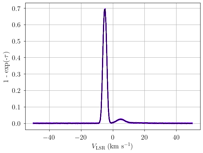
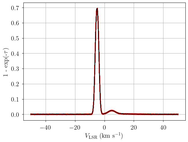
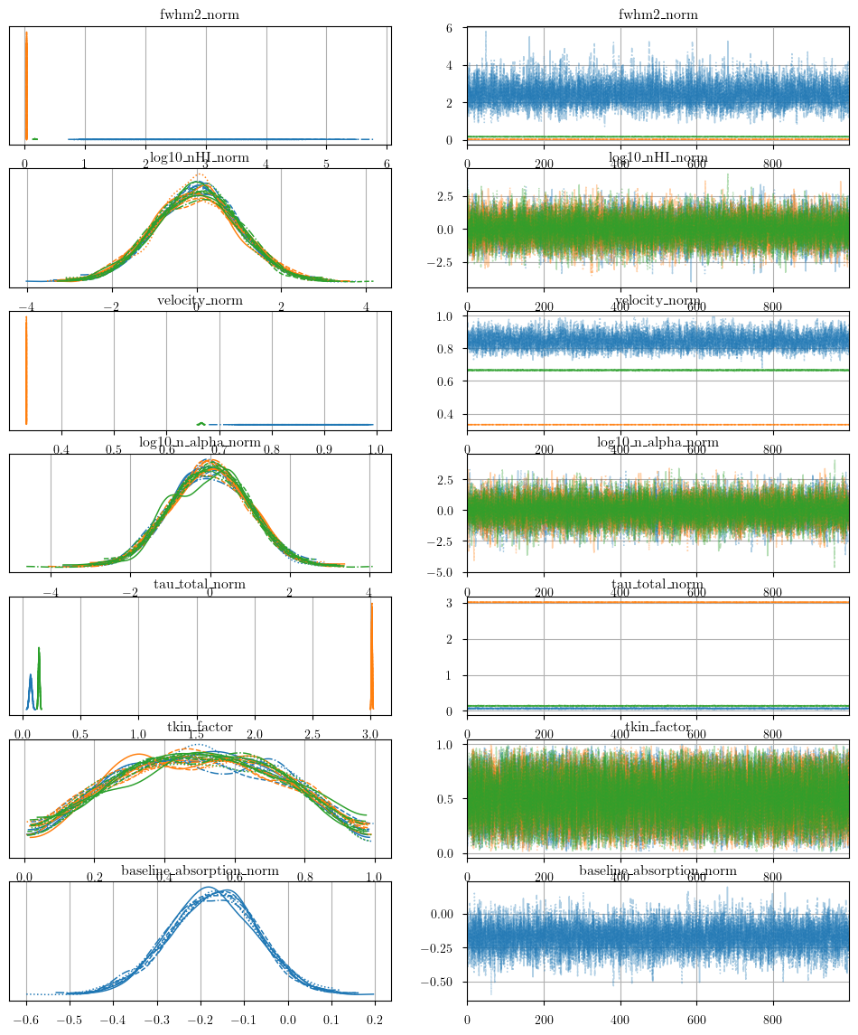
We generate posterior predictive checks as well as a trace plot of the individual chains. In the posterior predictive plot, we show each chain as a different color. Each line is one posterior sample.
[21]:
posterior = model.sample_posterior_predictive(
    thin=10, # keep one in {thin} posterior samples
)
_ = plot_predictive(model.data, posterior.posterior_predictive)
Sampling: [absorption]
[22]:
from bayes_spec.plots import plot_traces

_ = plot_traces(model.trace.solution_0, model.cloud_freeRVs + model.baseline_freeRVs + model.hyper_freeRVs)
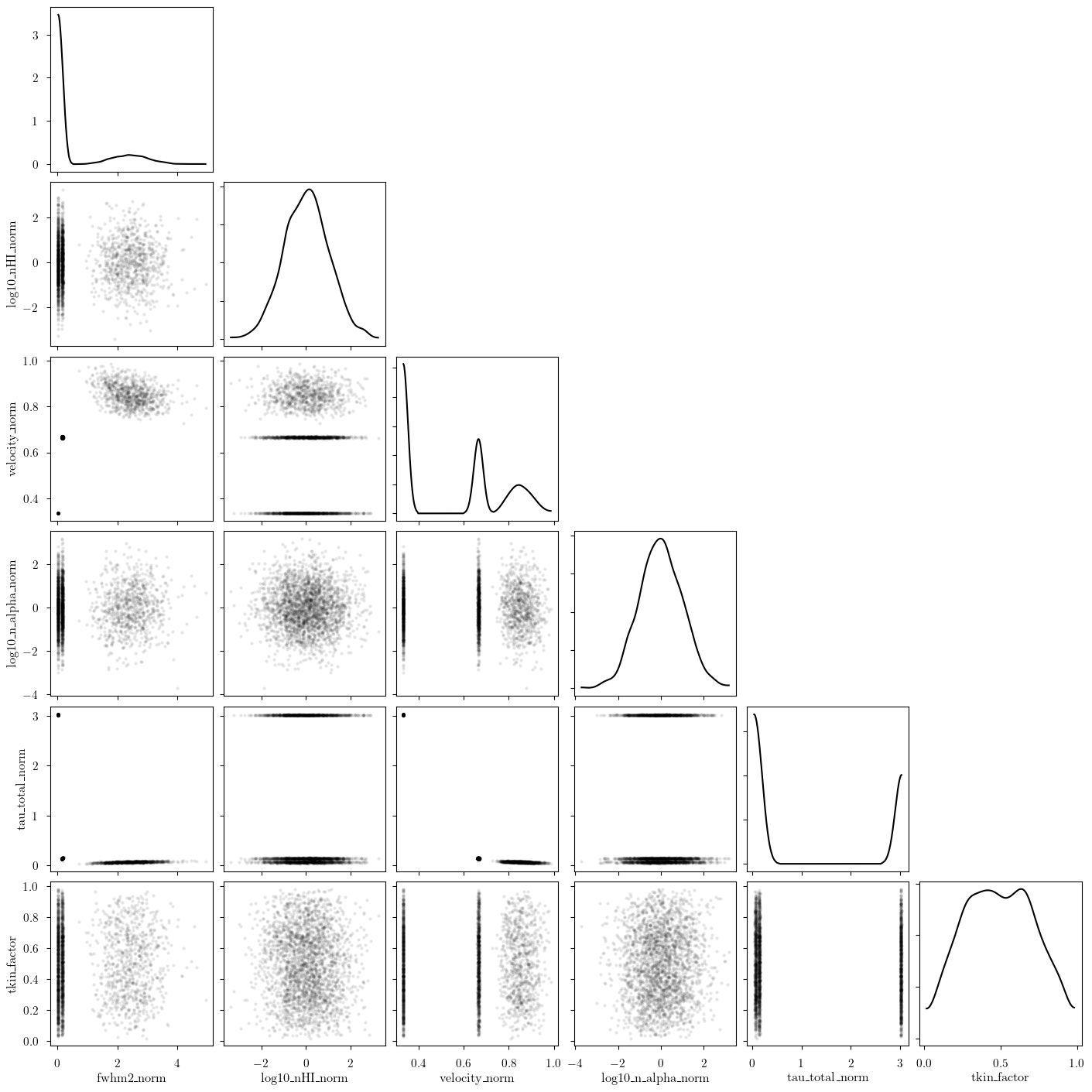
We can inspect the posterior distribution pair plots. First, the free parameters for all clouds. Keep an eye out for any strong degeneracies or non-linear correlations. If present, then these features can cause the posterior sampling to be inefficient. It may be worth re-parameterizing your model to remove these effects. Alternatively, increasing tune and target_accept can help.
[23]:
_ = plot_pair(
    model.trace.solution_0.sel(draw=slice(None, None, 10)), # samples
    model.cloud_freeRVs, # var_names to plot
    combine_dims=["cloud"], # concatenate clouds
    kind="scatter", # plot type
)
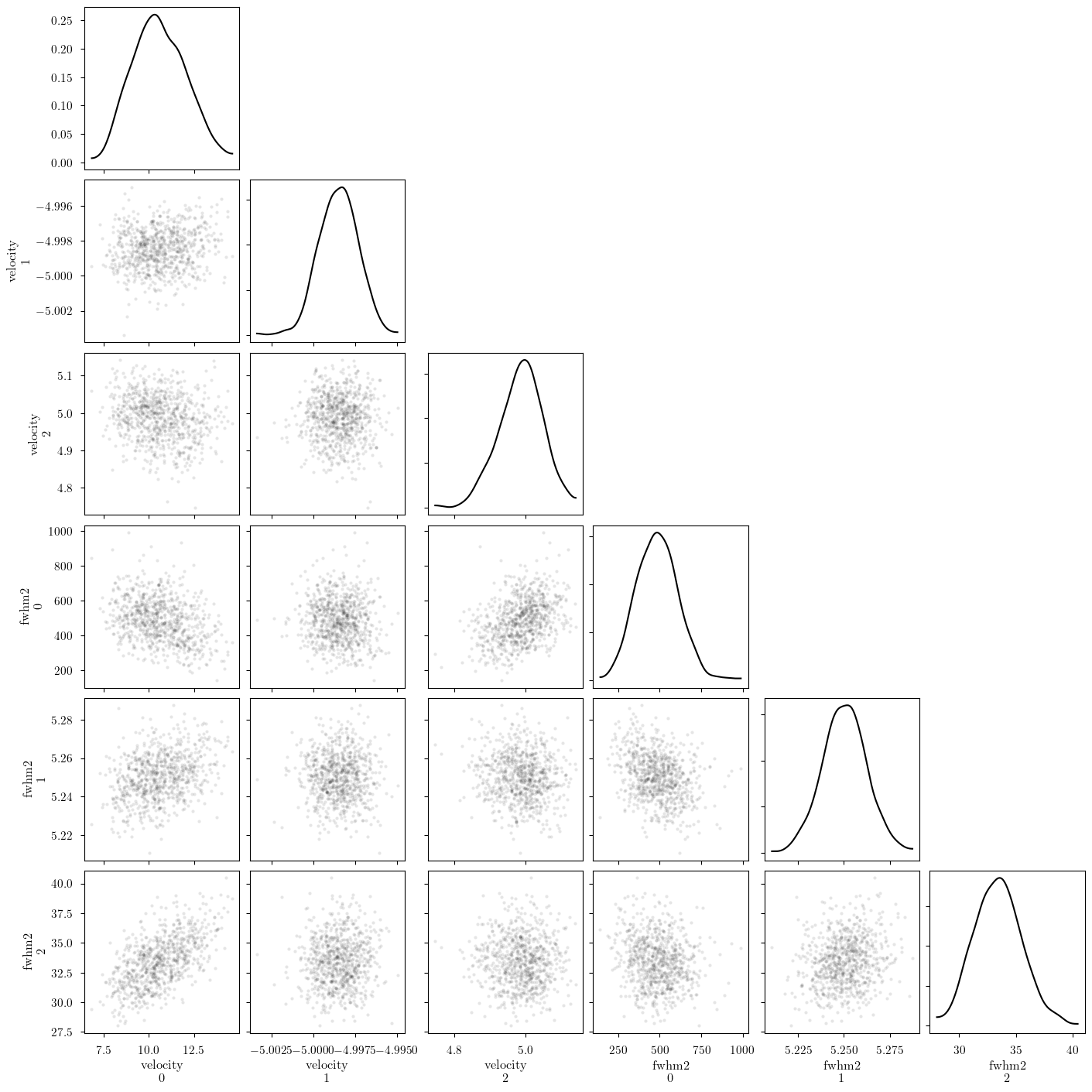
[24]:
_ = plot_pair(
    model.trace.solution_0.sel(draw=slice(None, None, 10)), # samples
    ["velocity", "fwhm2"], # var_names to plot
    combine_dims=None, # do not concatenate clouds
    kind="scatter", # plot type
)
[25]:
_ = plot_pair(
    model.trace.solution_0.sel(cloud=0, draw=slice(None, None, 10)), # samples
    model.cloud_freeRVs + model.hyper_freeRVs + model.baseline_freeRVs, # var_names to plot
    kind="scatter", # plot type
)
[26]:
_ = plot_pair(
    model.trace.solution_0.sel(cloud=1, draw=slice(None, None, 10)), # samples
    model.cloud_freeRVs + model.hyper_freeRVs + model.baseline_freeRVs, # var_names to plot
    kind="scatter", # plot type
)
[27]:
_ = plot_pair(
    model.trace.solution_0.sel(cloud=2, draw=slice(None, None, 10)), # samples
    model.cloud_freeRVs + model.hyper_freeRVs + model.baseline_freeRVs, # var_names to plot
    kind="scatter", # plot type
)
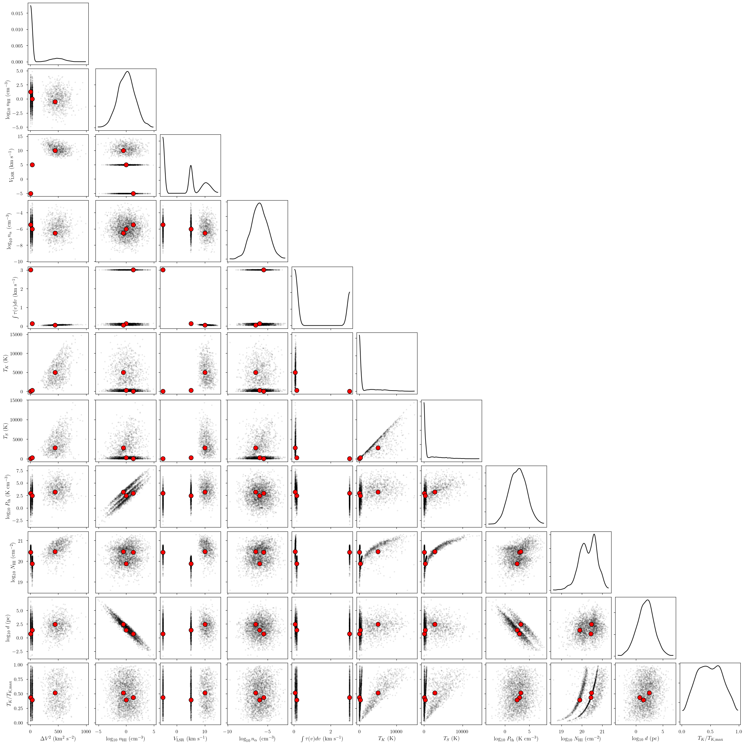
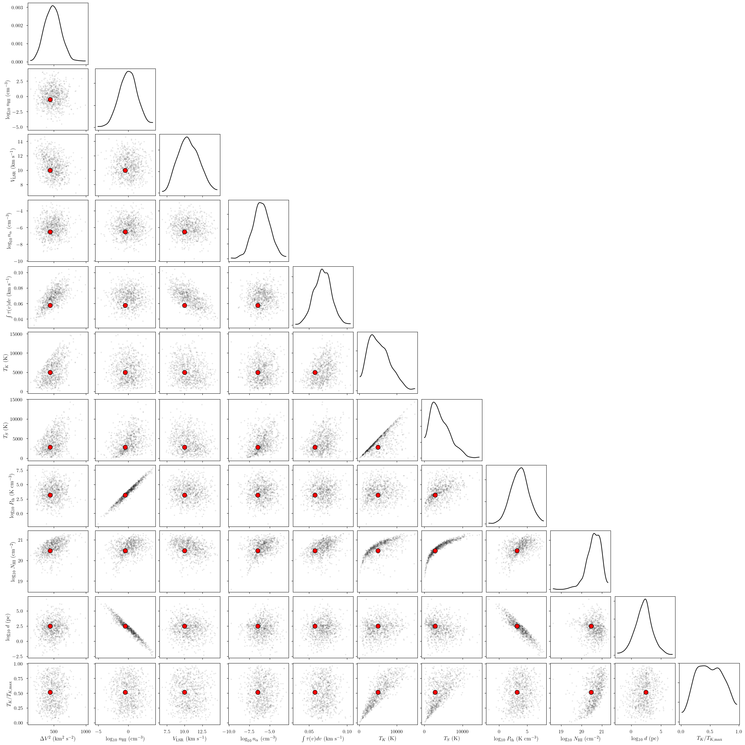
The red points represent the simulation parameters for the deterministic quantities.
[28]:
_ = plot_pair(
    model.trace.solution_0.sel(draw=slice(None, None, 10)), # samples
    var_names, # var_names to plot
    combine_dims=["cloud"], # concatenate clouds
    labeller=model.labeller, # label manager
    kind="scatter", # plot type
    reference_values=sim_params, # truths
)
[29]:
# identify simulation cloud corresponding to each posterior cloud
sim_cloud_map = {}
for i in range(n_clouds):
    posterior_velocity = model.trace.solution_0['velocity'].sel(cloud=i).data.mean()
    match = np.argmin(np.abs(sim_params["velocity"] - posterior_velocity))
    sim_cloud_map[i] = match
sim_cloud_map
[29]:
{0: np.int64(2), 1: np.int64(0), 2: np.int64(1)}
[30]:
print("cloud freeRVs", model.cloud_freeRVs)
print("cloud deterministics", model.cloud_deterministics)
print("hyper freeRVs", model.hyper_freeRVs)
print("hyper deterministics", model.hyper_deterministics)
cloud freeRVs ['fwhm2_norm', 'log10_nHI_norm', 'velocity_norm', 'log10_n_alpha_norm', 'tau_total_norm', 'tkin_factor']
cloud deterministics ['fwhm2', 'log10_nHI', 'velocity', 'log10_n_alpha', 'tau_total', 'tkin', 'tspin', 'log10_Pth', 'log10_NHI', 'log10_depth']
hyper freeRVs []
hyper deterministics []
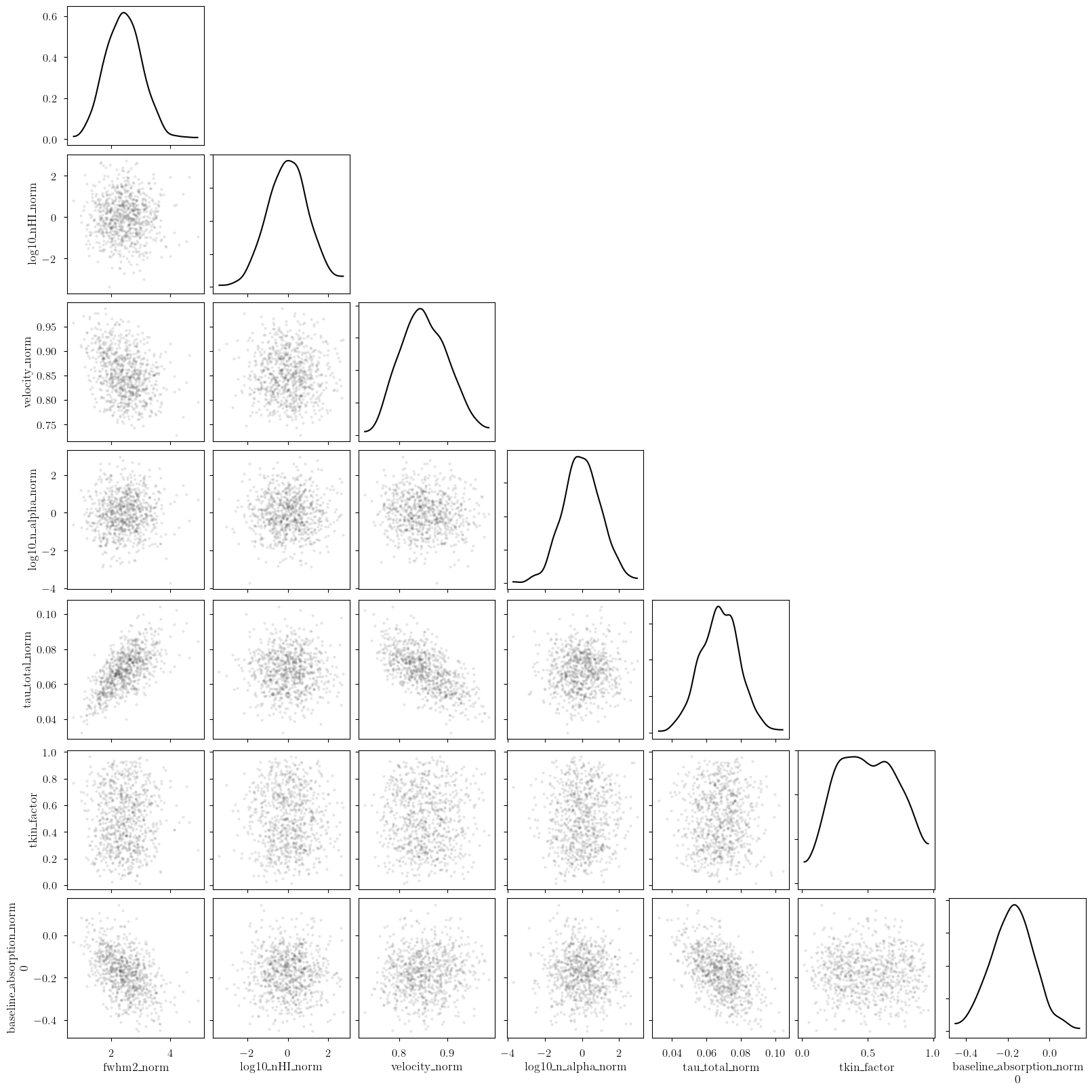
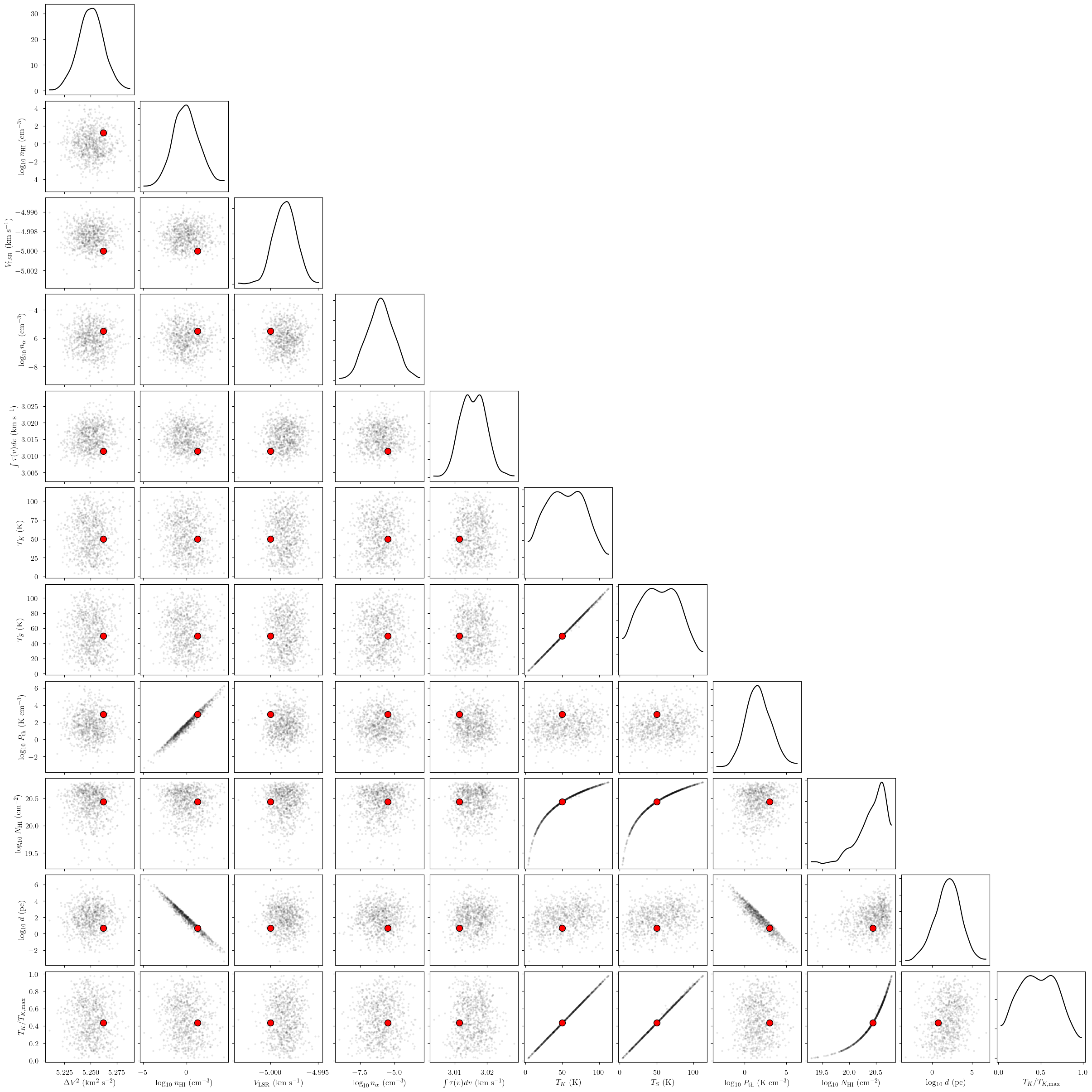
[31]:
cloud = 0

# subset of sim_params
my_sim_params = {}
for var_name in var_names:
    my_sim_params[var_name] = sim_params[var_name][sim_cloud_map[cloud]]

_ = plot_pair(
    model.trace.solution_0.sel(cloud=cloud, draw=slice(None, None, 10)), # samples
    var_names, # var_names to plot
    labeller=model.labeller, # label manager
    kind="scatter", # plot type
    reference_values=my_sim_params, # truths
)
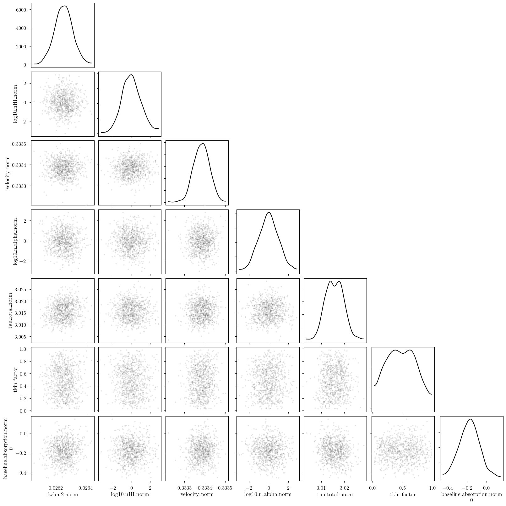
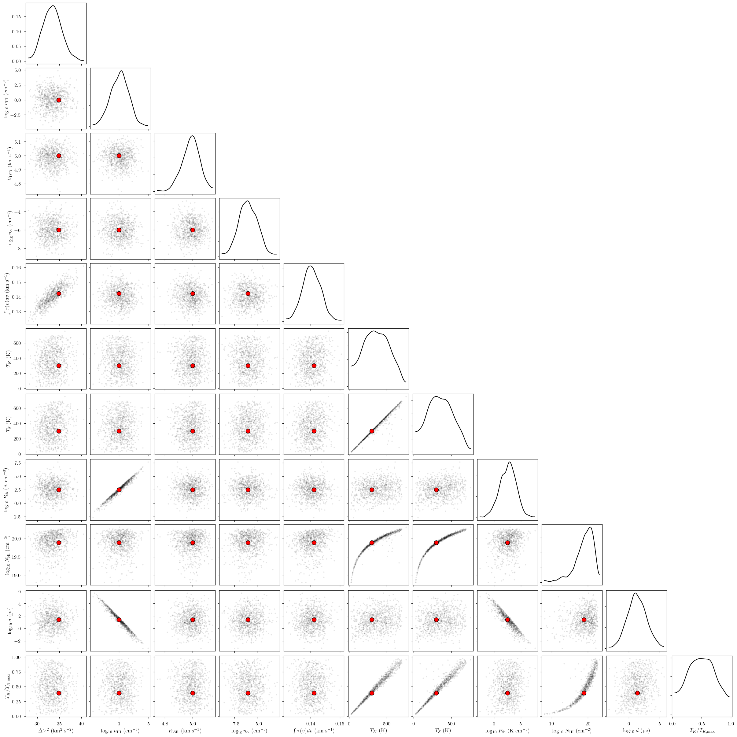
[32]:
cloud = 1

# subset of sim_params
my_sim_params = {}
for var_name in var_names:
    my_sim_params[var_name] = sim_params[var_name][sim_cloud_map[cloud]]

_ = plot_pair(
    model.trace.solution_0.sel(cloud=cloud, draw=slice(None, None, 10)), # samples
    var_names, # var_names to plot
    labeller=model.labeller, # label manager
    kind="scatter", # plot type
    reference_values=my_sim_params, # truths
)
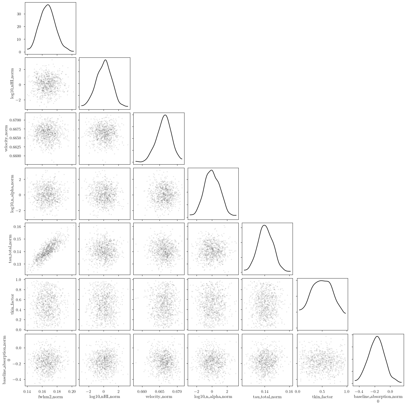
[33]:
cloud = 2

# subset of sim_params
my_sim_params = {}
for var_name in var_names:
    my_sim_params[var_name] = sim_params[var_name][sim_cloud_map[cloud]]

_ = plot_pair(
    model.trace.solution_0.sel(cloud=cloud, draw=slice(None, None, 10)), # samples
    var_names, # var_names to plot
    labeller=model.labeller, # label manager
    kind="scatter", # plot type
    reference_values=my_sim_params, # truths
)
Finally, we can get the posterior statistics, Bayesian Information Criterion (BIC), etc.
[34]:
point_stats = az.summary(model.trace.solution_0, kind='stats')
print("BIC:", model.bic())
display(point_stats)
BIC: -2090.8815371954106
| mean | sd | hdi_3% | hdi_97% | |
|---|---|---|---|---|
| baseline_absorption_norm[0] | -0.172 | 0.102 | -0.373 | 0.013 |
| log10_nHI_norm[0] | 0.005 | 0.982 | -1.853 | 1.832 |
| log10_nHI_norm[1] | -0.005 | 1.028 | -1.890 | 1.963 |
| log10_nHI_norm[2] | 0.007 | 0.991 | -1.857 | 1.831 |
| log10_n_alpha_norm[0] | -0.016 | 0.990 | -1.879 | 1.772 |
| log10_n_alpha_norm[1] | -0.007 | 0.990 | -1.804 | 1.862 |
| log10_n_alpha_norm[2] | 0.001 | 0.991 | -1.862 | 1.811 |
| fwhm2_norm[0] | 2.436 | 0.619 | 1.333 | 3.606 |
| fwhm2_norm[1] | 0.026 | 0.000 | 0.026 | 0.026 |
| fwhm2_norm[2] | 0.166 | 0.010 | 0.148 | 0.186 |
| velocity_norm[0] | 0.849 | 0.048 | 0.764 | 0.941 |
| velocity_norm[1] | 0.333 | 0.000 | 0.333 | 0.333 |
| velocity_norm[2] | 0.666 | 0.002 | 0.662 | 0.670 |
| tau_total_norm[0] | 0.068 | 0.011 | 0.047 | 0.089 |
| tau_total_norm[1] | 3.016 | 0.004 | 3.009 | 3.023 |
| tau_total_norm[2] | 0.140 | 0.006 | 0.129 | 0.152 |
| tkin_factor[0] | 0.499 | 0.225 | 0.117 | 0.906 |
| tkin_factor[1] | 0.499 | 0.228 | 0.110 | 0.909 |
| tkin_factor[2] | 0.501 | 0.225 | 0.096 | 0.892 |
| fwhm2[0] | 487.114 | 123.880 | 266.594 | 721.296 |
| fwhm2[1] | 5.251 | 0.012 | 5.227 | 5.273 |
| fwhm2[2] | 33.297 | 2.038 | 29.601 | 37.174 |
| log10_nHI[0] | 0.008 | 1.474 | -2.780 | 2.748 |
| log10_nHI[1] | -0.007 | 1.542 | -2.834 | 2.944 |
| log10_nHI[2] | 0.010 | 1.487 | -2.786 | 2.747 |
| velocity[0] | 10.483 | 1.434 | 7.915 | 13.238 |
| velocity[1] | -4.999 | 0.001 | -5.001 | -4.996 |
| velocity[2] | 4.989 | 0.059 | 4.874 | 5.098 |
| log10_n_alpha[0] | -6.016 | 0.990 | -7.879 | -4.228 |
| log10_n_alpha[1] | -6.007 | 0.990 | -7.804 | -4.138 |
| log10_n_alpha[2] | -5.999 | 0.991 | -7.862 | -4.189 |
| tau_total[0] | 0.068 | 0.011 | 0.047 | 0.089 |
| tau_total[1] | 3.016 | 0.004 | 3.009 | 3.023 |
| tau_total[2] | 0.140 | 0.006 | 0.129 | 0.152 |
| tkin[0] | 5316.642 | 2841.337 | 499.442 | 10387.527 |
| tkin[1] | 57.310 | 26.192 | 11.528 | 103.134 |
| tkin[2] | 364.451 | 164.902 | 55.951 | 641.153 |
| tspin[0] | 4116.224 | 2515.129 | 174.324 | 8680.417 |
| tspin[1] | 57.079 | 26.030 | 12.646 | 103.730 |
| tspin[2] | 354.046 | 160.308 | 55.412 | 628.097 |
| log10_Pth[0] | 3.657 | 1.504 | 0.899 | 6.594 |
| log10_Pth[1] | 1.687 | 1.561 | -1.362 | 4.478 |
| log10_Pth[2] | 2.509 | 1.512 | -0.201 | 5.394 |
| log10_NHI[0] | 20.602 | 0.353 | 19.941 | 21.206 |
| log10_NHI[1] | 20.433 | 0.267 | 19.944 | 20.791 |
| log10_NHI[2] | 19.894 | 0.266 | 19.408 | 20.289 |
| log10_depth[0] | 2.104 | 1.393 | -0.548 | 4.764 |
| log10_depth[1] | 1.950 | 1.568 | -1.121 | 4.801 |
| log10_depth[2] | 1.394 | 1.498 | -1.250 | 4.354 |
[ ]: