EmissionAbsorptionModel Constant Column Density Bias

Trey V. Wenger (c) July 2025

The default behavior of EmissionAbsorptionModel is to assume that the column density probed by absorption is identical to the column density probed by emission. This is the behavior when prior_sigma_log10_NHI is None (the default).

Here we demonstrate the bias imposed by assuming prior_sigma_log10_NHI = None.

# General imports
import time

import matplotlib.pyplot as plt
import arviz as az
import pandas as pd
import numpy as np
import pymc as pm

print("pymc version:", pm.__version__)
print("arviz version:", az.__version__)

import bayes_spec
print("bayes_spec version:", bayes_spec.__version__)

import caribou_hi
print("caribou_hi version:", caribou_hi.__version__)

# Notebook configuration
pd.options.display.max_rows = None

pymc version: 5.22.0
arviz version: 0.22.0dev
bayes_spec version: 1.9.0
caribou_hi version: 4.1.0+3.g94a913e.dirty

Simulating Data

from bayes_spec import SpecData

# spectral axes definitions
emission_axis = np.linspace(-60.0, 60.0, 200)  # km s-1
absorption_axis = np.linspace(-30.0, 30.0, 100)  # km s-1

# data noise can either be a scalar (assumed constant noise across the spectrum)
# or an array of the same length as the data
rms_emission = 0.1  # K
rms_absorption = 0.001  # 1 - exp(-tau)

# brightness data. In this case, we just throw in some random data for now
# since we are only doing this in order to simulate some actual data.
emission = rms_emission * np.random.randn(len(emission_axis))
absorption = rms_absorption * np.random.randn(len(absorption_axis))

dummy_data = {
    "emission": SpecData(
        emission_axis,
        emission,
        rms_emission,
        xlabel=r"$V_{\rm LSR}$ (km s$^{-1}$)",
        ylabel=r"$T_B$ (K)",
    ),
    "absorption": SpecData(
        absorption_axis,
        absorption,
        rms_absorption,
        xlabel=r"$V_{\rm LSR}$ (km s$^{-1}$)",
        ylabel=r"1 - exp(-$\tau$)",
    ),
}

# Plot dummy data
fig, axes = plt.subplots(2, layout="constrained", sharex=True)
axes[0].plot(dummy_data["emission"].spectral, dummy_data["emission"].brightness, "k-")
axes[0].plot(dummy_data["emission"].spectral, dummy_data["emission"].noise, "r-")
axes[1].plot(dummy_data["absorption"].spectral, dummy_data["absorption"].brightness, "k-", label="Data")
axes[1].plot(dummy_data["absorption"].spectral, dummy_data["absorption"].noise, "r-", label="Noise")
axes[1].set_xlabel(dummy_data["emission"].xlabel)
axes[0].set_ylabel(dummy_data["emission"].ylabel)
axes[1].set_ylabel(dummy_data["absorption"].ylabel)
_ = axes[1].legend(loc="lower left")

from caribou_hi import EmissionAbsorptionModel

# Initialize and define the model
n_clouds = 3
baseline_degree = 0
model = EmissionAbsorptionModel(
    dummy_data,
    n_clouds=n_clouds,
    baseline_degree=baseline_degree,
    bg_temp = 3.77, # assumed background temperature (K)
    seed=1234,
    verbose=True
)
model.add_priors(
    prior_filling_factor=[2.0, 1.0],  # filling factor prior shape
    prior_TB_fwhm=50.0, # peak brightness temperature x FWHM prior width (K km s-1)
    prior_tkin_factor=[2.0, 2.0], # kinetic temperature prior shape
    prior_sigma_log10_NHI=0.5, # log-normal column density distribution width
    prior_fwhm2=200.0, # FWHM^2 prior width (km2 s-2)
    prior_log10_nHI=[0.0, 1.5],  # log10(density) prior mean and width (cm-3)
    prior_velocity=[-15.0, 15.0],  # lower and upper limit of velocity prior (km/s)
    prior_log10_n_alpha=[-6.0, 1.0],  # log10(n_alpha) prior width (cm-3)
    prior_fwhm_L=None,  # Assume Gaussian line profile
    prior_baseline_coeffs=None,  # Default baseline priors
)
model.add_likelihood()

from caribou_hi import physics

# Simulation parameters
filling_factor = np.array([0.2, 0.8, 1.0])
absorption_weight = np.array([0.9, 0.8, 1.0])

log10_nHI = np.array([1.25, 0.0, -0.5])
tkin = np.array([50.0, 300.0, 5000.0])
n_alpha = np.array([1.0e-6, 2.0e-6, 3.0e-6])
depth = np.array([5.0, 25.0, 300.0])
nth_fwhm_1pc = np.array([1.25, 1.75, 1.5])
depth_nth_fwhm_power = np.array([0.2, 0.3, 0.4])

tspin = physics.calc_spin_temp(tkin, 10.0**log10_nHI, n_alpha).eval()
print("tspin", tspin)

fwhm_nonthermal = physics.calc_nonthermal_fwhm(depth, nth_fwhm_1pc, depth_nth_fwhm_power)
fwhm2_thermal = physics.calc_thermal_fwhm2(tkin)
fwhm = np.sqrt(fwhm_nonthermal**2.0 + fwhm2_thermal)
print("fwhm", fwhm)

log10_Pth = np.log10(tkin) + log10_nHI
print("log10_Pth", log10_Pth)

log10_NHI = log10_nHI + np.log10(depth) + 18.489351
print("log10_NHI", log10_NHI)

tau_total = physics.calc_tau_total(10.0**log10_NHI, tspin)
print("tau_total", tau_total)

const = np.sqrt(2.0 * np.pi) / (2.0 * np.sqrt(2.0 * np.log(2.0)))
tau_peak = tau_total / fwhm / const
print("tau_peak", tau_peak)

TB_fwhm = filling_factor * tspin * (1.0 - np.exp(-tau_peak)) * fwhm
print("TB_fwhm", TB_fwhm)

wt_ff_tspin = absorption_weight / filling_factor / tspin
print("wt_ff_tspin", wt_ff_tspin)

sim_params = {
    "TB_fwhm": TB_fwhm,
    "tkin": tkin,
    "filling_factor": filling_factor,
    "wt_ff_tspin": wt_ff_tspin,
    "absorption_weight": absorption_weight,
    "fwhm2": fwhm**2.0,
    "log10_nHI": log10_nHI,
    "velocity": np.array([-5.0, 5.0, 10.0]),
    "n_alpha": n_alpha,
    "baseline_emission_norm": [0.0],
    "baseline_absorption_norm": [0.0],
}

# add derived quantities to sim_params
for key in model.cloud_deterministics:
    if key not in sim_params.keys():
        sim_params[key] = model.model[key].eval(sim_params, on_unused_input="ignore")

# Evaluate and save simulated observation
emission = model.model["emission"].eval(sim_params, on_unused_input="ignore")
absorption = model.model["absorption"].eval(sim_params, on_unused_input="ignore")

data = {
    "emission": SpecData(
        emission_axis,
        emission,
        rms_emission,
        xlabel=r"$V_{\rm LSR}$ (km s$^{-1}$)",
        ylabel=r"$T_B$ (K)",
    ),
    "absorption": SpecData(
        absorption_axis,
        absorption,
        rms_absorption,
        xlabel=r"$V_{\rm LSR}$ (km s$^{-1}$)",
        ylabel=r"1 - exp(-$\tau$)",
    ),
}

tspin [  49.97911226  298.78900835 4259.26982821]
fwhm [ 2.29393108  5.90364916 21.08270953]
log10_Pth [2.94897    2.47712125 3.19897   ]
log10_NHI [20.438321   19.88729101 20.46647225]
tau_total [3.01218479 0.14166923 0.03771258]
tau_peak [1.23358487 0.02254357 0.00168046]
TB_fwhm [ 16.25152201  31.45660514 150.77326269]
wt_ff_tspin [0.09003761 0.00334684 0.00023478]

sim_params

{'TB_fwhm': array([ 16.25152201,  31.45660514, 150.77326269]),
 'tkin': array([  50.,  300., 5000.]),
 'filling_factor': array([0.2, 0.8, 1. ]),
 'wt_ff_tspin': array([0.09003761, 0.00334684, 0.00023478]),
 'absorption_weight': array([0.9, 0.8, 1. ]),
 'fwhm2': array([  5.26211978,  34.85307344, 444.48064099]),
 'log10_nHI': array([ 1.25,  0.  , -0.5 ]),
 'velocity': array([-5.,  5., 10.]),
 'n_alpha': array([1.e-06, 2.e-06, 3.e-06]),
 'baseline_emission_norm': [0.0],
 'baseline_absorption_norm': [0.0],
 'log10_n_alpha': array([-5.39682159, -5.98007026, -5.53006719]),
 'tspin': array([  49.99361181,  297.82829201, 4250.13330217]),
 'tau_total': array([3.01046199, 0.14213143, 0.03779372]),
 'log10_Pth': array([2.94897   , 2.47712125, 3.19897   ]),
 'log10_NHI': array([20.43819852, 19.88730692, 20.46647304]),
 'log10_depth': array([0.69884752, 1.39795592, 2.47712204])}

# Plot data
fig, axes = plt.subplots(2, layout="constrained", sharex=True)
axes[0].plot(data["emission"].spectral, data["emission"].brightness, "k-")
axes[0].plot(data["emission"].spectral, data["emission"].noise, "r-")
axes[1].plot(data["absorption"].spectral, data["absorption"].brightness, "k-", label="Data")
axes[1].plot(data["absorption"].spectral, data["absorption"].noise, "r-", label="Noise")
axes[1].set_xlabel(data["emission"].xlabel)
axes[0].set_ylabel(data["emission"].ylabel)
axes[1].set_ylabel(data["absorption"].ylabel)
_ = axes[1].legend(loc="upper left")

Model Definition

Here we assume prior_sigma_log10_NHI = None.

# Initialize and define the model
model = EmissionAbsorptionModel(
    data,
    n_clouds=n_clouds,
    baseline_degree=baseline_degree,
    bg_temp = 3.77, # assumed background temperature (K)
    seed=1234,
    verbose=True
)
model.add_priors(
    prior_filling_factor=[2.0, 1.0],  # filling factor prior shape
    prior_TB_fwhm=200.0, # peak brightness temperature x FWHM prior width (K km s-1)
    prior_tkin_factor=[2.0, 2.0], # kinetic temperature prior shape
    prior_sigma_log10_NHI=None,
    prior_fwhm2=200.0, # FWHM^2 prior width (km2 s-2)
    prior_log10_nHI=[0.0, 1.5],  # log10(density) prior mean and width (cm-3)
    prior_velocity=[-20.0, 20.0],  # lower and upper limit of velocity prior (km/s)
    prior_log10_n_alpha=[-6.0, 1.0],  # log10(n_alpha) prior width (cm-3)
    prior_fwhm_L=None,  # Assume Gaussian line profile
    prior_baseline_coeffs=None,  # Default baseline priors
)
model.add_likelihood()

# model string representation
print(model.model.str_repr())

  baseline_emission_norm ~ Normal(0, 1)
baseline_absorption_norm ~ Normal(0, 1)
              fwhm2_norm ~ Gamma(0.5, f())
          log10_nHI_norm ~ Normal(0, 1)
           velocity_norm ~ Beta(2, 2)
      log10_n_alpha_norm ~ Normal(0, 1)
            TB_fwhm_norm ~ HalfNormal(0, 1)
        tkin_factor_norm ~ Beta(2, 2)
          filling_factor ~ Beta(2, 1)
                   fwhm2 ~ Deterministic(f(fwhm2_norm))
               log10_nHI ~ Deterministic(f(log10_nHI_norm))
                velocity ~ Deterministic(f(velocity_norm))
           log10_n_alpha ~ Deterministic(f(log10_n_alpha_norm))
                 TB_fwhm ~ Deterministic(f(TB_fwhm_norm))
                    tkin ~ Deterministic(f(tkin_factor_norm, fwhm2_norm, TB_fwhm_norm))
                   tspin ~ Deterministic(f(tkin_factor_norm, log10_n_alpha_norm, fwhm2_norm, TB_fwhm_norm, log10_nHI_norm))
               tau_total ~ Deterministic(f(fwhm2_norm, filling_factor, TB_fwhm_norm, tkin_factor_norm, log10_n_alpha_norm, log10_nHI_norm))
               log10_Pth ~ Deterministic(f(log10_nHI_norm, tkin_factor_norm, fwhm2_norm, TB_fwhm_norm))
               log10_NHI ~ Deterministic(f(fwhm2_norm, filling_factor, tkin_factor_norm, log10_n_alpha_norm, TB_fwhm_norm, log10_nHI_norm))
             log10_depth ~ Deterministic(f(log10_nHI_norm, fwhm2_norm, filling_factor, tkin_factor_norm, log10_n_alpha_norm, TB_fwhm_norm))
              absorption ~ Normal(f(baseline_absorption_norm, fwhm2_norm, velocity_norm, filling_factor, TB_fwhm_norm, tkin_factor_norm, log10_n_alpha_norm, log10_nHI_norm), <constant>)
                emission ~ Normal(f(filling_factor, baseline_emission_norm, tkin_factor_norm, fwhm2_norm, log10_n_alpha_norm, TB_fwhm_norm, log10_nHI_norm, velocity_norm), <constant>)

from bayes_spec.plots import plot_predictive

# prior predictive check
prior = model.sample_prior_predictive(
    samples=1000,  # prior predictive samples
)
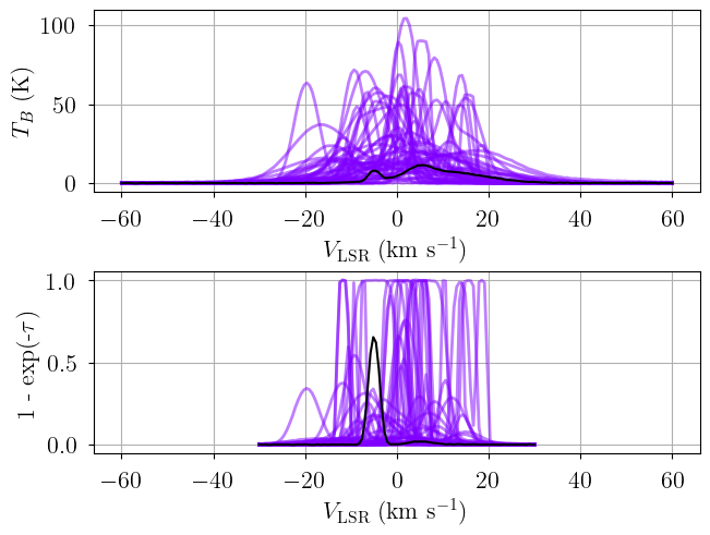
axes = plot_predictive(model.data, prior.prior_predictive.sel(draw=slice(None, None, 20)))
axes.ravel()[1].sharex(axes.ravel()[0])

Sampling: [TB_fwhm_norm, absorption, baseline_absorption_norm, baseline_emission_norm, emission, filling_factor, fwhm2_norm, log10_nHI_norm, log10_n_alpha_norm, tkin_factor_norm, velocity_norm]

print(model.cloud_freeRVs)
print(model.cloud_deterministics)

['fwhm2_norm', 'log10_nHI_norm', 'velocity_norm', 'log10_n_alpha_norm', 'TB_fwhm_norm', 'tkin_factor_norm', 'filling_factor']
['fwhm2', 'log10_nHI', 'velocity', 'log10_n_alpha', 'TB_fwhm', 'tkin', 'tspin', 'tau_total', 'log10_Pth', 'log10_NHI', 'log10_depth']

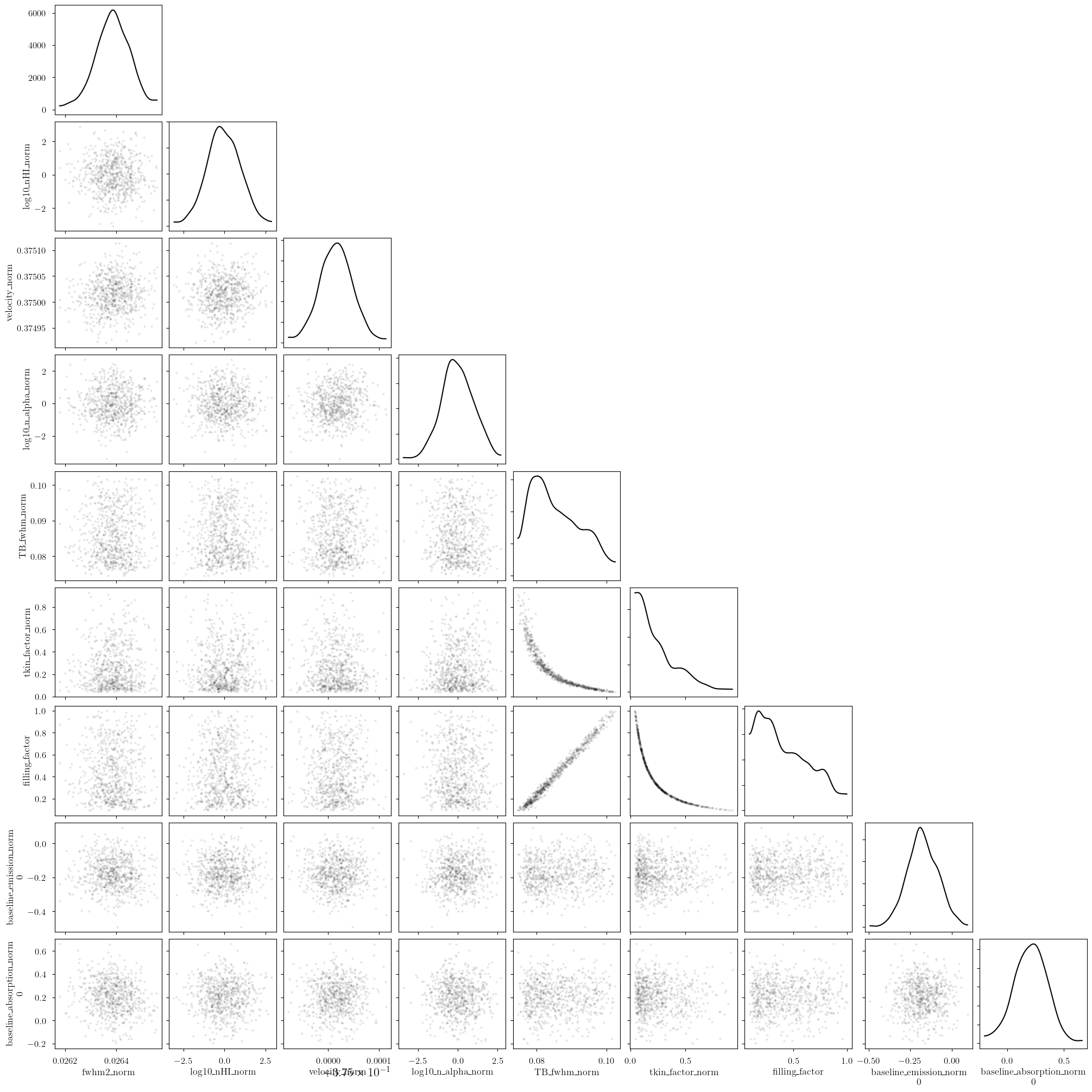
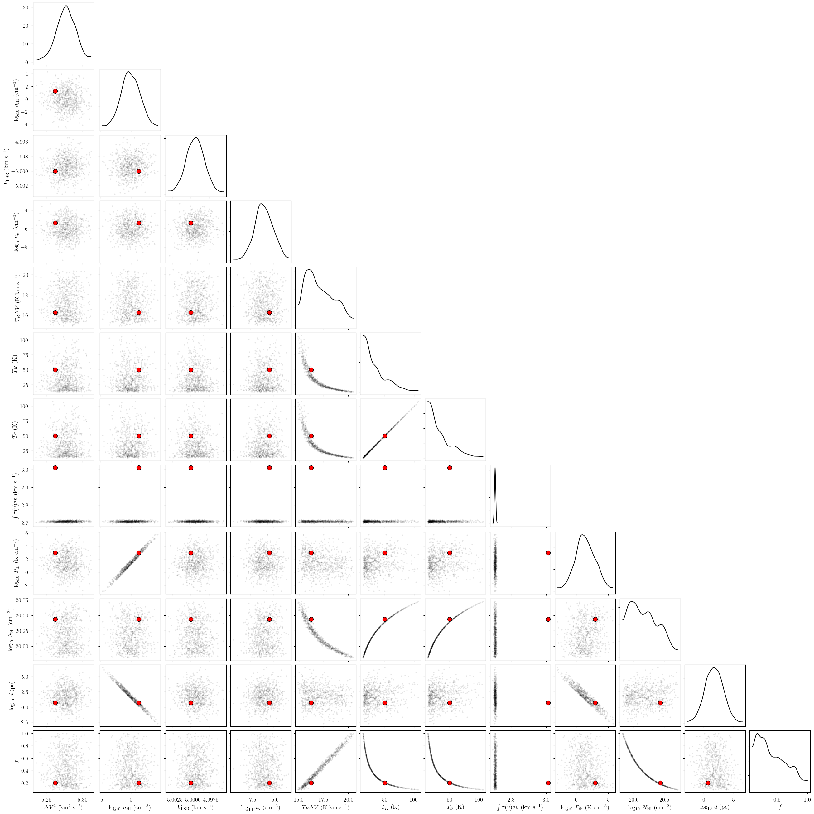
from bayes_spec.plots import plot_pair

var_names = model.cloud_deterministics + [p for p in model.cloud_freeRVs if "_norm" not in p]
print(var_names)
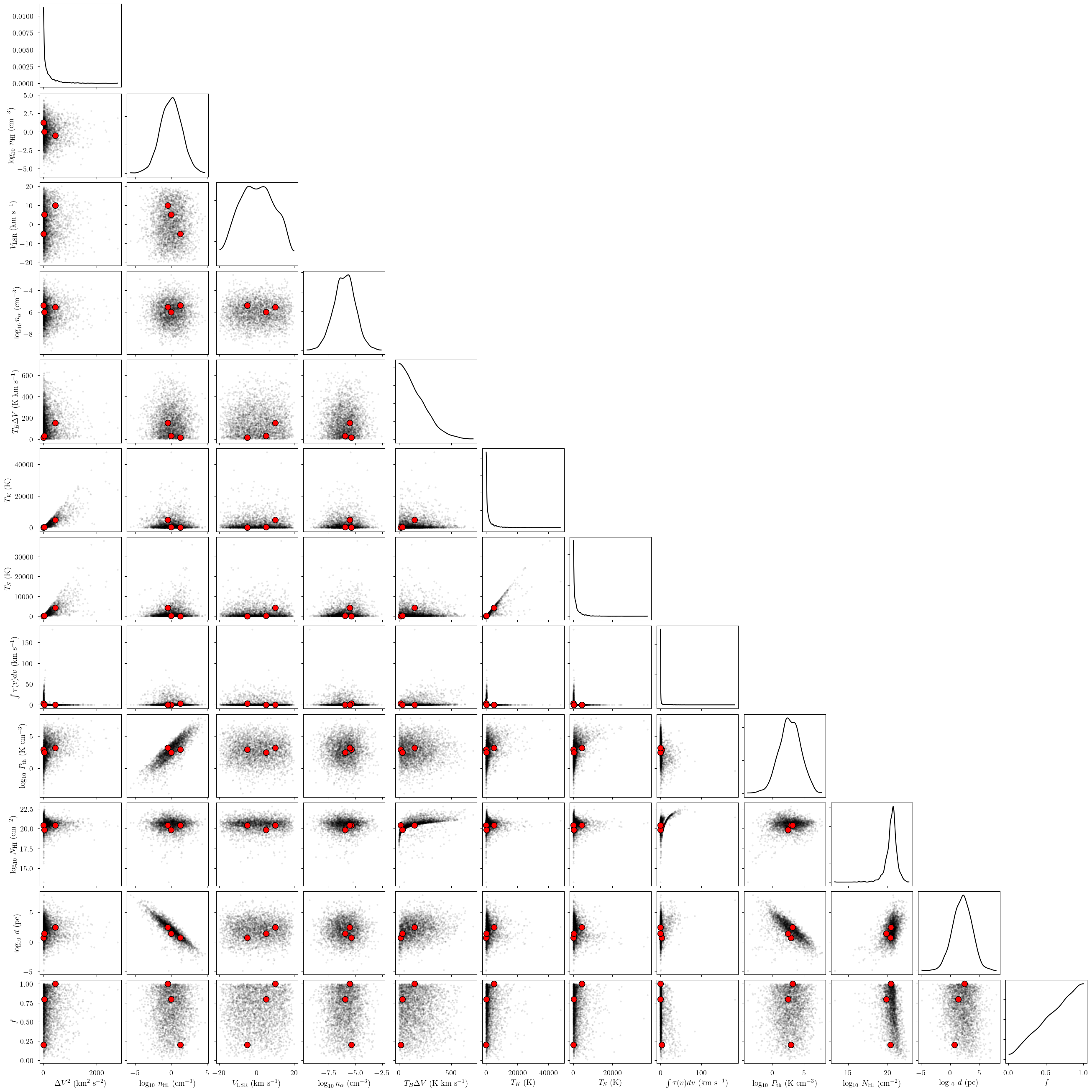
_ = plot_pair(
    prior.prior, # samples
    var_names, # var_names to plot
    combine_dims=["cloud"], # concatenate clouds
    labeller=model.labeller, # label manager
    kind="scatter", # plot type
    reference_values=sim_params, # truths
)

['fwhm2', 'log10_nHI', 'velocity', 'log10_n_alpha', 'TB_fwhm', 'tkin', 'tspin', 'tau_total', 'log10_Pth', 'log10_NHI', 'log10_depth', 'filling_factor']

Variational Inference

start = time.time()
model.fit(
    n = 1_000_000, # maximum number of VI iterations
    draws = 1_000, # number of posterior samples
    rel_tolerance = 0.005, # VI relative convergence threshold
    abs_tolerance = 0.005, # VI absolute convergence threshold
    learning_rate = 0.001, # VI learning rate
    start = {"velocity_norm": np.linspace(0.1, 0.9, n_clouds)},
)
end = time.time()
print(f"Runtime: {(end-start)/60.0:.2f} minutes")

Convergence achieved at 69400
Interrupted at 69,399 [6%]: Average Loss = 2.369e+05

Adding log-likelihood to trace

Runtime: 1.62 minutes

pm.summary(model.trace.posterior)

arviz - WARNING - Shape validation failed: input_shape: (1, 1000), minimum_shape: (chains=2, draws=4)

	mean	sd	hdi_3%	hdi_97%	mcse_mean	mcse_sd	ess_bulk	ess_tail	r_hat
baseline_emission_norm[0]	-0.166	0.071	-0.290	-0.029	0.002	0.002	1099.0	975.0	NaN
baseline_absorption_norm[0]	0.253	0.101	0.082	0.458	0.003	0.002	889.0	907.0	NaN
log10_nHI_norm[0]	0.781	0.547	-0.135	1.907	0.017	0.012	1026.0	950.0	NaN
log10_nHI_norm[1]	0.050	1.039	-1.723	2.036	0.031	0.021	1113.0	1117.0	NaN
log10_nHI_norm[2]	0.156	0.971	-1.741	1.954	0.034	0.024	829.0	766.0	NaN
log10_n_alpha_norm[0]	0.330	0.885	-1.283	2.047	0.028	0.024	966.0	974.0	NaN
log10_n_alpha_norm[1]	0.383	0.771	-1.188	1.739	0.024	0.017	1051.0	944.0	NaN
log10_n_alpha_norm[2]	0.373	0.711	-0.874	1.763	0.023	0.016	984.0	974.0	NaN
fwhm2_norm[0]	2.218	0.014	2.190	2.243	0.000	0.000	1130.0	651.0	NaN
fwhm2_norm[1]	0.026	0.000	0.026	0.026	0.000	0.000	1084.0	982.0	NaN
fwhm2_norm[2]	0.170	0.002	0.166	0.173	0.000	0.000	892.0	916.0	NaN
velocity_norm[0]	0.751	0.001	0.749	0.753	0.000	0.000	1030.0	852.0	NaN
velocity_norm[1]	0.375	0.000	0.375	0.375	0.000	0.000	984.0	905.0	NaN
velocity_norm[2]	0.625	0.001	0.624	0.626	0.000	0.000	779.0	693.0	NaN
TB_fwhm_norm[0]	0.755	0.002	0.752	0.759	0.000	0.000	872.0	909.0	NaN
TB_fwhm_norm[1]	0.090	0.000	0.090	0.090	0.000	0.000	933.0	766.0	NaN
TB_fwhm_norm[2]	0.155	0.001	0.153	0.157	0.000	0.000	996.0	860.0	NaN
tkin_factor_norm[0]	0.613	0.081	0.473	0.776	0.003	0.002	962.0	871.0	NaN
tkin_factor_norm[1]	0.116	0.000	0.116	0.116	0.000	0.000	831.0	902.0	NaN
tkin_factor_norm[2]	0.439	0.009	0.423	0.456	0.000	0.000	1017.0	994.0	NaN
filling_factor[0]	0.880	0.081	0.721	0.985	0.003	0.003	1015.0	773.0	NaN
filling_factor[1]	0.577	0.000	0.576	0.578	0.000	0.000	934.0	879.0	NaN
filling_factor[2]	0.905	0.019	0.871	0.941	0.001	0.000	934.0	981.0	NaN
fwhm2[0]	443.673	2.799	437.980	448.685	0.084	0.065	1130.0	651.0	NaN
fwhm2[1]	5.277	0.004	5.268	5.284	0.000	0.000	1084.0	982.0	NaN
fwhm2[2]	33.943	0.409	33.208	34.665	0.014	0.010	892.0	916.0	NaN
log10_nHI[0]	1.172	0.821	-0.202	2.861	0.026	0.019	1026.0	950.0	NaN
log10_nHI[1]	0.075	1.558	-2.584	3.054	0.047	0.032	1113.0	1117.0	NaN
log10_nHI[2]	0.234	1.456	-2.611	2.931	0.051	0.036	829.0	766.0	NaN
velocity[0]	10.032	0.035	9.973	10.106	0.001	0.001	1030.0	852.0	NaN
velocity[1]	-4.999	0.001	-5.002	-4.997	0.000	0.000	984.0	905.0	NaN
velocity[2]	5.002	0.024	4.957	5.046	0.001	0.001	779.0	693.0	NaN
log10_n_alpha[0]	-5.670	0.885	-7.283	-3.953	0.028	0.024	966.0	974.0	NaN
log10_n_alpha[1]	-5.617	0.771	-7.188	-4.261	0.024	0.017	1051.0	944.0	NaN
log10_n_alpha[2]	-5.627	0.711	-6.874	-4.237	0.023	0.016	984.0	974.0	NaN
TB_fwhm[0]	151.048	0.419	150.327	151.893	0.014	0.010	872.0	909.0	NaN
TB_fwhm[1]	18.008	0.018	17.971	18.040	0.001	0.000	933.0	766.0	NaN
TB_fwhm[2]	31.071	0.211	30.657	31.453	0.007	0.005	996.0	860.0	NaN
tkin[0]	5949.124	782.265	4591.947	7521.248	25.146	17.366	967.0	840.0	NaN
tkin[1]	20.297	0.017	20.267	20.328	0.001	0.000	1023.0	976.0	NaN
tkin[2]	328.874	7.667	315.184	343.851	0.242	0.165	996.0	917.0	NaN
tspin[0]	5629.971	848.895	3894.574	6942.667	26.522	22.241	1038.0	983.0	NaN
tspin[1]	20.294	0.019	20.259	20.327	0.001	0.001	1038.0	926.0	NaN
tspin[2]	326.490	9.696	310.197	341.878	0.295	0.814	1057.0	979.0	NaN
tau_total[0]	0.034	0.008	0.023	0.045	0.000	0.001	1058.0	983.0	NaN
tau_total[1]	2.709	0.007	2.697	2.721	0.000	0.000	1055.0	944.0	NaN
tau_total[2]	0.113	0.005	0.105	0.120	0.000	0.000	1076.0	952.0	NaN
log10_Pth[0]	4.943	0.822	3.599	6.671	0.025	0.018	1053.0	853.0	NaN
log10_Pth[1]	1.382	1.558	-1.277	4.362	0.047	0.032	1112.0	1119.0	NaN
log10_Pth[2]	2.750	1.456	-0.083	5.454	0.051	0.036	829.0	765.0	NaN
log10_NHI[0]	20.525	0.043	20.472	20.608	0.001	0.002	1028.0	769.0	NaN
log10_NHI[1]	20.001	0.001	19.999	20.002	0.000	0.000	1019.0	949.0	NaN
log10_NHI[2]	19.827	0.010	19.811	19.847	0.000	0.000	964.0	975.0	NaN
log10_depth[0]	0.863	0.821	-0.817	2.260	0.025	0.019	1037.0	872.0	NaN
log10_depth[1]	1.437	1.558	-1.542	4.096	0.047	0.032	1112.0	1119.0	NaN
log10_depth[2]	1.105	1.457	-1.593	3.948	0.051	0.036	830.0	766.0	NaN

posterior = model.sample_posterior_predictive(
    thin=10,  # keep one in {thin} posterior samples
)
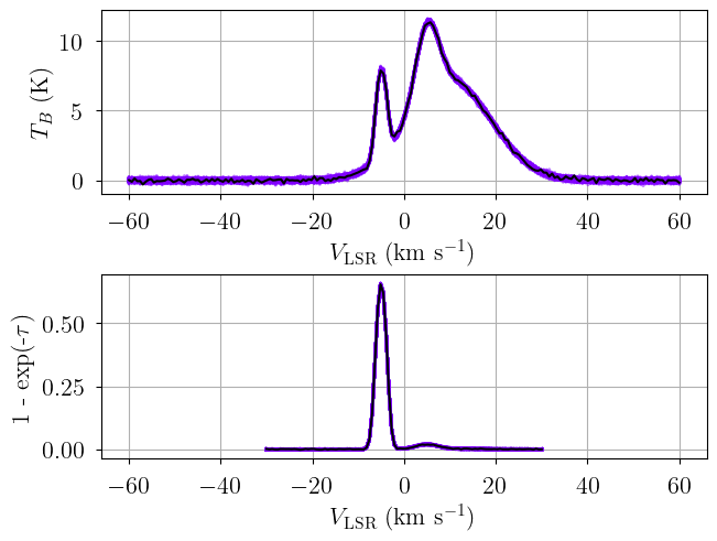
axes = plot_predictive(model.data, posterior.posterior_predictive)
axes.ravel()[1].sharex(axes.ravel()[0])

Sampling: [absorption, emission]

Posterior Sampling: MCMC

start = time.time()
model.sample(
    init="advi+adapt_diag",  # initialization strategy
    tune=1000,  # tuning samples
    draws=1000,  # posterior samples
    chains=8,  # number of independent chains
    cores=8,  # number of parallel chains
    init_kwargs={
        "rel_tolerance": 0.005,
        "abs_tolerance": 0.005,
        "learning_rate": 0.001,
        "start": {"velocity_norm": np.linspace(0.1, 0.9, n_clouds)},
    },  # VI initialization arguments
    nuts_kwargs={"target_accept": 0.9},  # NUTS arguments
)
end = time.time()
print(f"Runtime: {(end-start)/60.0:.2f} minutes")

Initializing NUTS using custom advi+adapt_diag strategy

Convergence achieved at 69400
Interrupted at 69,399 [6%]: Average Loss = 2.369e+05
Multiprocess sampling (8 chains in 8 jobs)
NUTS: [baseline_emission_norm, baseline_absorption_norm, fwhm2_norm, log10_nHI_norm, velocity_norm, log10_n_alpha_norm, TB_fwhm_norm, tkin_factor_norm, filling_factor]

Sampling 8 chains for 1_000 tune and 1_000 draw iterations (8_000 + 8_000 draws total) took 355 seconds.

Adding log-likelihood to trace

Runtime: 7.62 minutes

model.solve(
    init_params="random_from_data", # GMM initialization strategy
    n_init=10, # number of GMM initilizations
    max_iter=1_000, # maximum number of GMM iterations
    kl_div_threshold=0.1, # covergence threshold
)

GMM converged to unique solution
7 of 8 chains appear converged.

print("solutions:", model.solutions)
az.summary(model.trace["solution_0"])
# this also works: az.summary(model.trace.solution_0)

solutions: [0]

	mean	sd	hdi_3%	hdi_97%	mcse_mean	mcse_sd	ess_bulk	ess_tail	r_hat
baseline_emission_norm[0]	-0.175	0.089	-0.343	-0.008	0.004	0.002	619.0	1289.0	1.01
baseline_absorption_norm[0]	0.208	0.142	-0.047	0.489	0.005	0.003	695.0	1383.0	1.01
log10_nHI_norm[0]	0.243	0.918	-1.477	2.017	0.042	0.022	474.0	892.0	1.02
log10_nHI_norm[1]	-0.044	0.989	-1.986	1.742	0.031	0.018	1036.0	1791.0	1.00
log10_nHI_norm[2]	0.054	0.976	-1.929	1.789	0.034	0.018	834.0	1402.0	1.01
log10_n_alpha_norm[0]	0.323	0.992	-1.695	2.051	0.047	0.025	461.0	756.0	1.03
log10_n_alpha_norm[1]	-0.022	0.991	-1.834	1.854	0.034	0.018	839.0	1380.0	1.01
log10_n_alpha_norm[2]	0.037	0.957	-1.737	1.849	0.036	0.019	719.0	1264.0	1.02
fwhm2_norm[0]	2.218	0.022	2.178	2.260	0.001	0.000	542.0	1217.0	1.01
fwhm2_norm[1]	0.026	0.000	0.026	0.027	0.000	0.000	859.0	1249.0	1.00
fwhm2_norm[2]	0.170	0.005	0.160	0.178	0.000	0.000	285.0	869.0	1.03
velocity_norm[0]	0.751	0.002	0.748	0.754	0.000	0.000	265.0	643.0	1.03
velocity_norm[1]	0.375	0.000	0.375	0.375	0.000	0.000	914.0	1475.0	1.00
velocity_norm[2]	0.625	0.001	0.624	0.626	0.000	0.000	659.0	1277.0	1.01
TB_fwhm_norm[0]	0.756	0.005	0.747	0.765	0.000	0.000	259.0	610.0	1.02
TB_fwhm_norm[1]	0.086	0.007	0.076	0.098	0.001	0.000	178.0	474.0	1.04
TB_fwhm_norm[2]	0.155	0.003	0.149	0.161	0.000	0.000	236.0	572.0	1.03
tkin_factor_norm[0]	0.651	0.139	0.406	0.905	0.007	0.003	449.0	508.0	1.02
tkin_factor_norm[1]	0.257	0.189	0.041	0.624	0.013	0.008	182.0	449.0	1.03
tkin_factor_norm[2]	0.558	0.129	0.385	0.808	0.007	0.004	308.0	747.0	1.04
filling_factor[0]	0.800	0.133	0.564	0.999	0.005	0.002	642.0	800.0	1.01
filling_factor[1]	0.430	0.235	0.094	0.846	0.018	0.007	182.0	453.0	1.03
filling_factor[2]	0.765	0.152	0.515	0.999	0.009	0.003	241.0	301.0	1.05
fwhm2[0]	443.591	4.423	435.516	451.967	0.190	0.089	542.0	1217.0	1.01
fwhm2[1]	5.277	0.013	5.253	5.302	0.000	0.000	859.0	1249.0	1.00
fwhm2[2]	33.906	0.970	32.018	35.649	0.057	0.023	285.0	869.0	1.03
log10_nHI[0]	0.364	1.377	-2.215	3.026	0.063	0.034	474.0	892.0	1.02
log10_nHI[1]	-0.066	1.483	-2.979	2.613	0.046	0.027	1036.0	1791.0	1.00
log10_nHI[2]	0.081	1.464	-2.894	2.683	0.051	0.027	834.0	1402.0	1.01
velocity[0]	10.026	0.062	9.907	10.145	0.004	0.002	265.0	643.0	1.03
velocity[1]	-4.999	0.001	-5.002	-4.997	0.000	0.000	914.0	1475.0	1.00
velocity[2]	5.001	0.027	4.952	5.052	0.001	0.000	659.0	1277.0	1.01
log10_n_alpha[0]	-5.677	0.992	-7.695	-3.949	0.047	0.025	461.0	756.0	1.03
log10_n_alpha[1]	-6.022	0.991	-7.834	-4.146	0.034	0.018	839.0	1380.0	1.01
log10_n_alpha[2]	-5.963	0.957	-7.737	-4.151	0.036	0.019	719.0	1264.0	1.02
TB_fwhm[0]	151.120	0.990	149.327	153.046	0.062	0.029	259.0	610.0	1.02
TB_fwhm[1]	17.151	1.377	15.137	19.651	0.107	0.042	178.0	474.0	1.04
TB_fwhm[2]	30.930	0.649	29.730	32.171	0.042	0.019	236.0	572.0	1.03
tkin[0]	6313.761	1350.128	3816.781	8669.615	63.114	26.768	451.0	528.0	1.02
tkin[1]	35.288	20.113	13.199	74.426	1.401	0.828	182.0	442.0	1.03
tkin[2]	415.529	95.228	286.631	595.766	5.088	2.978	274.0	544.0	1.05
tspin[0]	5658.773	1200.468	3448.713	7805.614	48.752	21.505	603.0	1140.0	1.01
tspin[1]	35.198	19.992	13.174	74.098	1.393	0.819	182.0	442.0	1.03
tspin[2]	404.744	90.470	285.950	575.953	4.890	3.042	275.0	612.0	1.04
tau_total[0]	0.038	0.007	0.026	0.051	0.000	0.000	1067.0	1938.0	1.00
tau_total[1]	2.709	0.004	2.702	2.715	0.000	0.000	4852.0	5301.0	1.00
tau_total[2]	0.112	0.003	0.106	0.118	0.000	0.000	1383.0	3010.0	1.00
log10_Pth[0]	4.154	1.371	1.484	6.699	0.063	0.033	482.0	898.0	1.02
log10_Pth[1]	1.419	1.494	-1.398	4.247	0.047	0.026	1027.0	1849.0	1.00
log10_Pth[2]	2.689	1.463	-0.206	5.354	0.051	0.027	828.0	1483.0	1.01
log10_NHI[0]	20.571	0.078	20.468	20.718	0.003	0.002	658.0	859.0	1.01
log10_NHI[1]	20.178	0.227	19.815	20.563	0.017	0.006	182.0	442.0	1.03
log10_NHI[2]	19.908	0.092	19.774	20.073	0.005	0.002	252.0	379.0	1.05
log10_depth[0]	1.718	1.371	-0.888	4.323	0.064	0.035	467.0	806.0	1.02
log10_depth[1]	1.755	1.506	-1.170	4.528	0.050	0.029	927.0	1568.0	1.01
log10_depth[2]	1.338	1.462	-1.377	4.175	0.051	0.027	832.0	1274.0	1.01

posterior = model.sample_posterior_predictive(
    thin=10,  # keep one in {thin} posterior samples
)
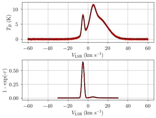
axes = plot_predictive(model.data, posterior.posterior_predictive)
axes.ravel()[0].sharex(axes.ravel()[1])

Sampling: [absorption, emission]

from bayes_spec.plots import plot_traces

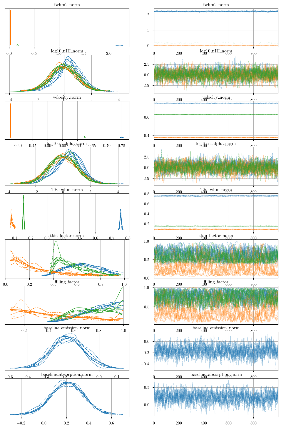
_ = plot_traces(model.trace.posterior, model.cloud_freeRVs + model.baseline_freeRVs + model.hyper_freeRVs)

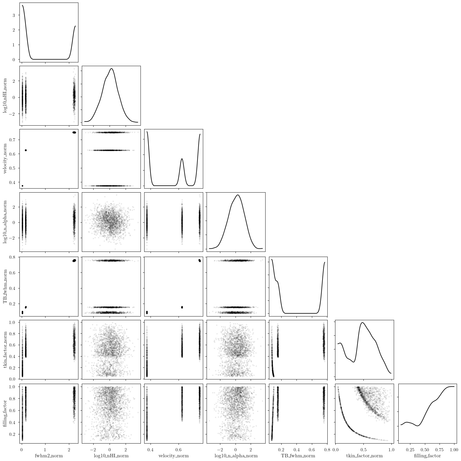
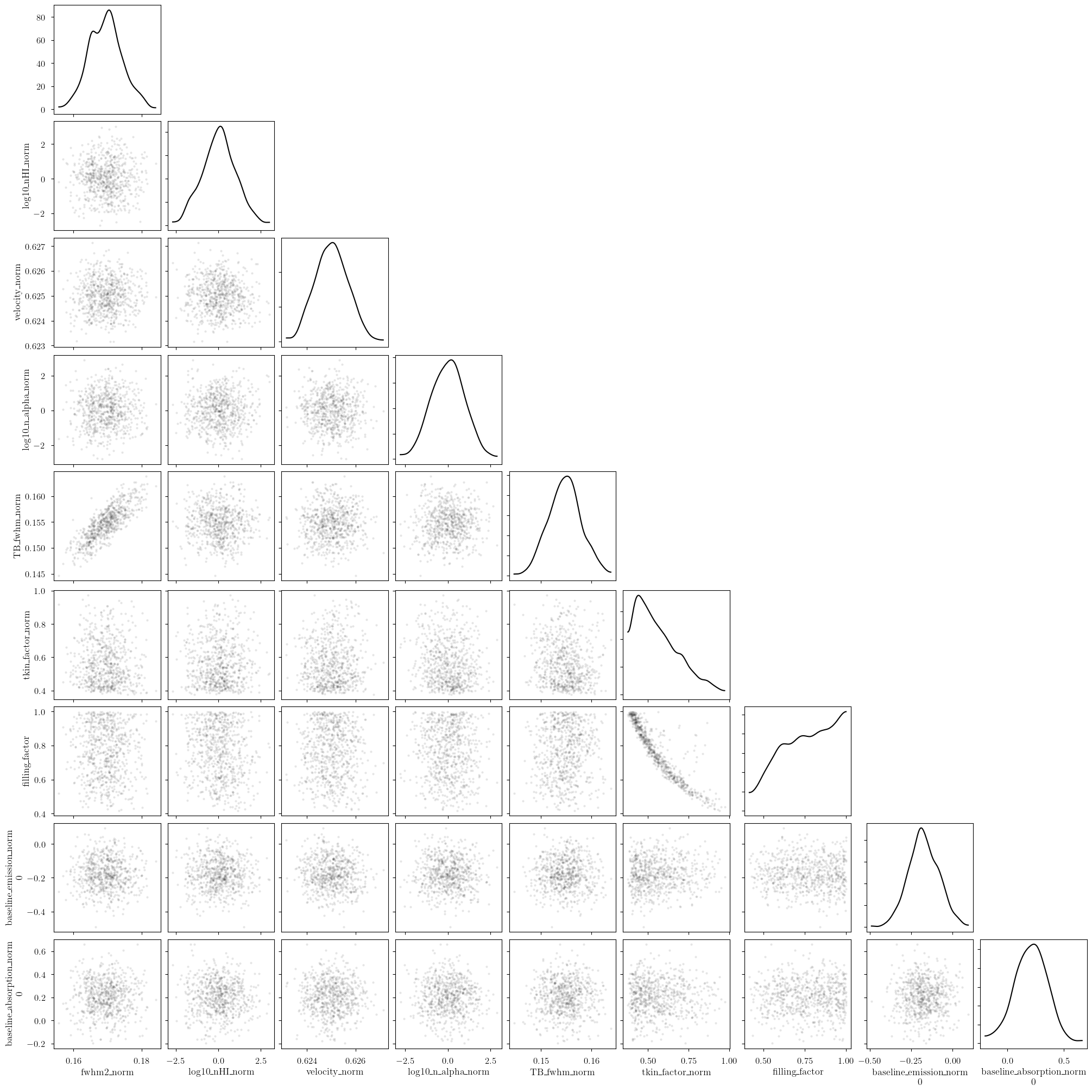
_ = plot_pair(
    model.trace.solution_0.sel(draw=slice(None, None, 10)), # samples
    model.cloud_freeRVs, # var_names to plot
    combine_dims=["cloud"], # concatenate clouds
    kind="scatter", # plot type
)

_ = plot_pair(
    model.trace.solution_0.sel(draw=slice(None, None, 10)), # samples
    ["velocity", "fwhm2"], # var_names to plot
    combine_dims=None, # do not concatenate clouds
    kind="scatter", # plot type
)

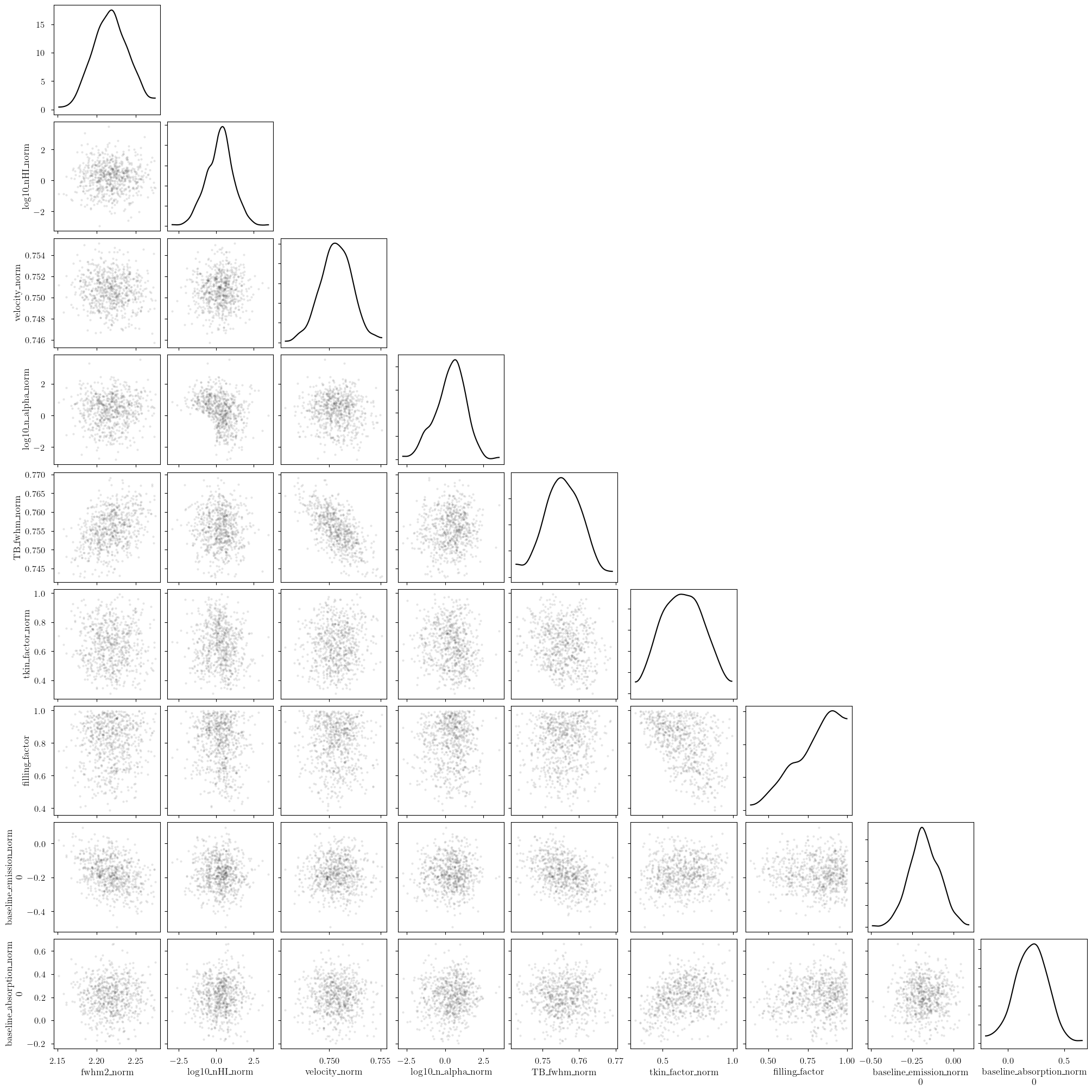
_ = plot_pair(
    model.trace.solution_0.sel(cloud=0, draw=slice(None, None, 10)), # samples
    model.cloud_freeRVs + model.hyper_freeRVs + model.baseline_freeRVs, # var_names to plot
    kind="scatter", # plot type
)

_ = plot_pair(
    model.trace.solution_0.sel(cloud=1, draw=slice(None, None, 10)), # samples
    model.cloud_freeRVs + model.hyper_freeRVs + model.baseline_freeRVs, # var_names to plot
    kind="scatter", # plot type
)

_ = plot_pair(
    model.trace.solution_0.sel(cloud=2, draw=slice(None, None, 10)), # samples
    model.cloud_freeRVs + model.hyper_freeRVs + model.baseline_freeRVs, # var_names to plot
    kind="scatter", # plot type
)

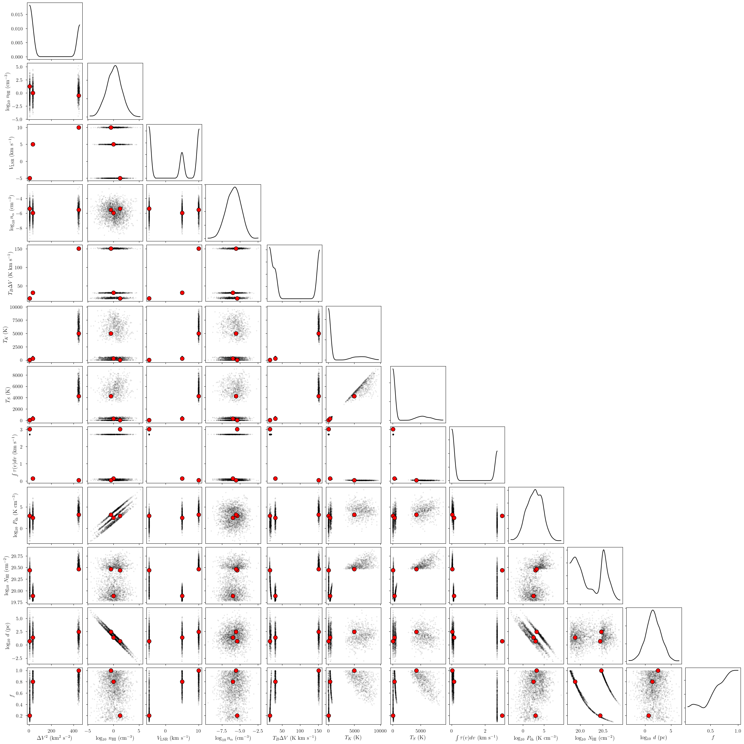
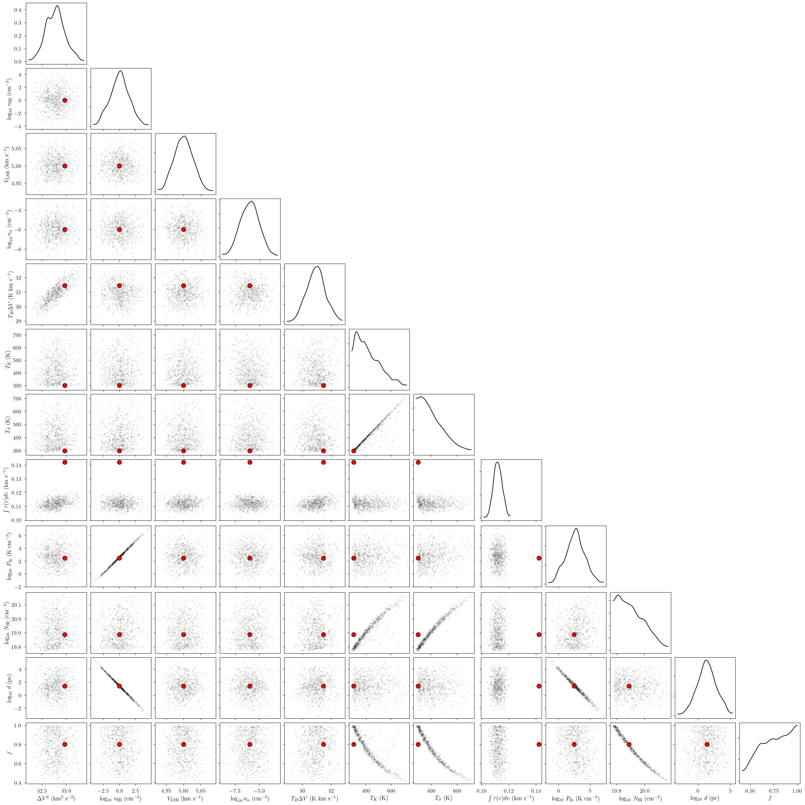
_ = plot_pair(
    model.trace.solution_0.sel(draw=slice(None, None, 10)), # samples
    var_names, # var_names to plot
    combine_dims=["cloud"], # concatenate clouds
    labeller=model.labeller, # label manager
    kind="scatter", # plot type
    reference_values=sim_params, # truths
)

# identify simulation cloud corresponding to each posterior cloud
sim_cloud_map = {}
for i in range(n_clouds):
    posterior_velocity = model.trace.solution_0['velocity'].sel(cloud=i).data.mean()
    match = np.argmin(np.abs(sim_params["velocity"] - posterior_velocity))
    sim_cloud_map[i] = match
sim_cloud_map

{0: np.int64(2), 1: np.int64(0), 2: np.int64(1)}

print("cloud freeRVs", model.cloud_freeRVs)
print("cloud deterministics", model.cloud_deterministics)
print("hyper freeRVs", model.hyper_freeRVs)
print("hyper deterministics", model.hyper_deterministics)

cloud freeRVs ['fwhm2_norm', 'log10_nHI_norm', 'velocity_norm', 'log10_n_alpha_norm', 'TB_fwhm_norm', 'tkin_factor_norm', 'filling_factor']
cloud deterministics ['fwhm2', 'log10_nHI', 'velocity', 'log10_n_alpha', 'TB_fwhm', 'tkin', 'tspin', 'tau_total', 'log10_Pth', 'log10_NHI', 'log10_depth']
hyper freeRVs []
hyper deterministics []

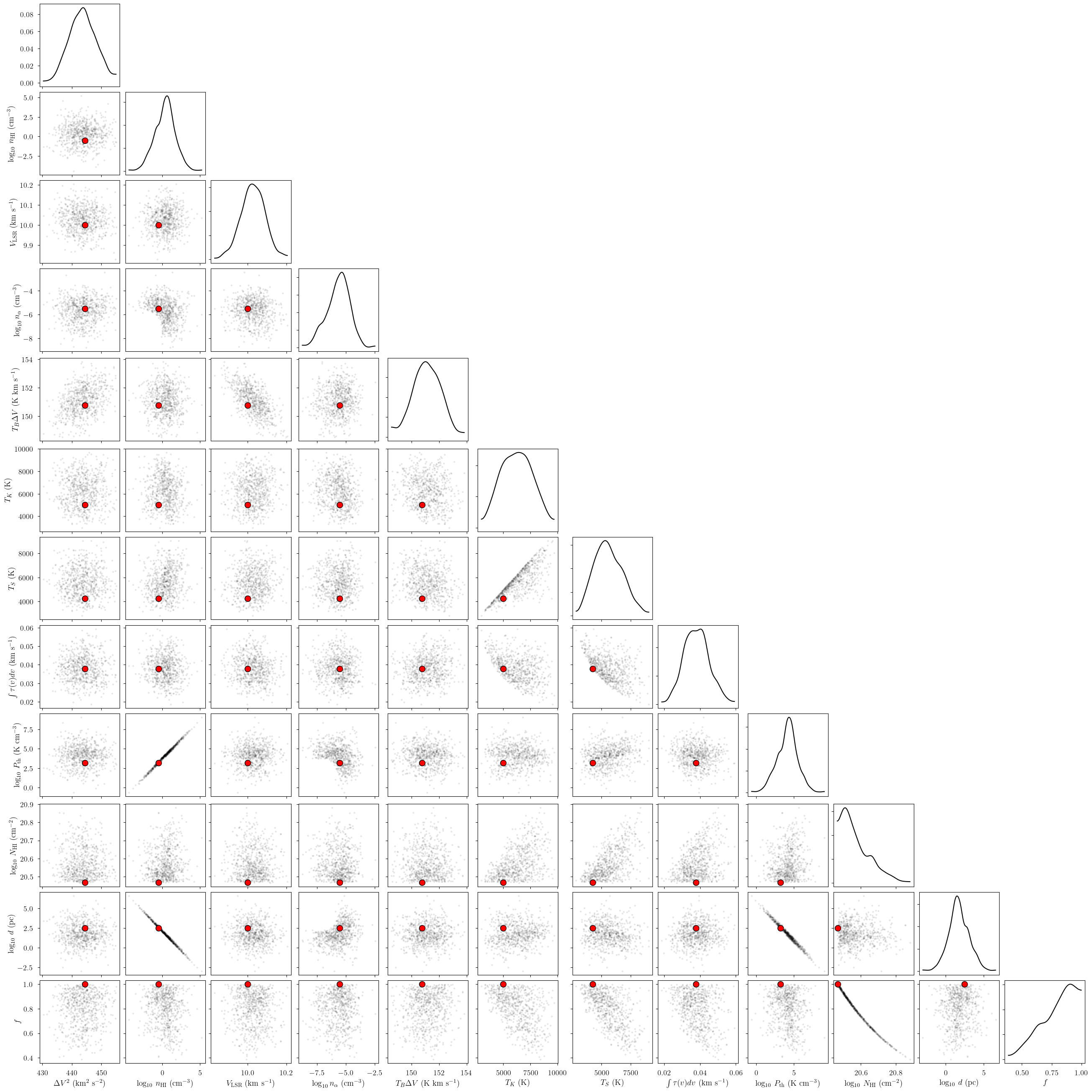
cloud = 0

# subset of sim_params
my_sim_params = {}
for var_name in var_names:
    my_sim_params[var_name] = sim_params[var_name][sim_cloud_map[cloud]]

_ = plot_pair(
    model.trace.solution_0.sel(cloud=cloud, draw=slice(None, None, 10)), # samples
    var_names, # var_names to plot
    labeller=model.labeller, # label manager
    kind="scatter", # plot type
    reference_values=my_sim_params, # truths
)

cloud = 1

# subset of sim_params
my_sim_params = {}
for var_name in var_names:
    my_sim_params[var_name] = sim_params[var_name][sim_cloud_map[cloud]]

_ = plot_pair(
    model.trace.solution_0.sel(cloud=cloud, draw=slice(None, None, 10)), # samples
    var_names, # var_names to plot
    labeller=model.labeller, # label manager
    kind="scatter", # plot type
    reference_values=my_sim_params, # truths
)

cloud = 2

# subset of sim_params
my_sim_params = {}
for var_name in var_names:
    my_sim_params[var_name] = sim_params[var_name][sim_cloud_map[cloud]]

_ = plot_pair(
    model.trace.solution_0.sel(cloud=cloud, draw=slice(None, None, 10)), # samples
    var_names, # var_names to plot
    labeller=model.labeller, # label manager
    kind="scatter", # plot type
    reference_values=my_sim_params, # truths
)

point_stats = az.summary(model.trace.solution_0, kind="stats", hdi_prob=0.68)
print("BIC:", model.bic())
display(point_stats)

BIC: -1320.5678665470405

	mean	sd	hdi_16%	hdi_84%
baseline_emission_norm[0]	-0.175	0.089	-0.265	-0.090
baseline_absorption_norm[0]	0.208	0.142	0.065	0.344
log10_nHI_norm[0]	0.243	0.918	-0.636	1.109
log10_nHI_norm[1]	-0.044	0.989	-1.039	0.890
log10_nHI_norm[2]	0.054	0.976	-0.825	1.097
log10_n_alpha_norm[0]	0.323	0.992	-0.534	1.385
log10_n_alpha_norm[1]	-0.022	0.991	-0.957	1.042
log10_n_alpha_norm[2]	0.037	0.957	-0.942	0.957
fwhm2_norm[0]	2.218	0.022	2.196	2.241
fwhm2_norm[1]	0.026	0.000	0.026	0.026
fwhm2_norm[2]	0.170	0.005	0.165	0.174
velocity_norm[0]	0.751	0.002	0.749	0.752
velocity_norm[1]	0.375	0.000	0.375	0.375
velocity_norm[2]	0.625	0.001	0.624	0.626
TB_fwhm_norm[0]	0.756	0.005	0.750	0.760
TB_fwhm_norm[1]	0.086	0.007	0.076	0.089
TB_fwhm_norm[2]	0.155	0.003	0.151	0.158
tkin_factor_norm[0]	0.651	0.139	0.493	0.792
tkin_factor_norm[1]	0.257	0.189	0.041	0.303
tkin_factor_norm[2]	0.558	0.129	0.393	0.608
filling_factor[0]	0.800	0.133	0.739	0.994
filling_factor[1]	0.430	0.235	0.096	0.538
filling_factor[2]	0.765	0.152	0.684	0.999
fwhm2[0]	443.591	4.423	439.295	448.211
fwhm2[1]	5.277	0.013	5.265	5.291
fwhm2[2]	33.906	0.970	32.923	34.853
log10_nHI[0]	0.364	1.377	-0.954	1.663
log10_nHI[1]	-0.066	1.483	-1.558	1.335
log10_nHI[2]	0.081	1.464	-1.237	1.646
velocity[0]	10.026	0.062	9.963	10.083
velocity[1]	-4.999	0.001	-5.001	-4.998
velocity[2]	5.001	0.027	4.974	5.027
log10_n_alpha[0]	-5.677	0.992	-6.534	-4.615
log10_n_alpha[1]	-6.022	0.991	-6.957	-4.958
log10_n_alpha[2]	-5.963	0.957	-6.942	-5.043
TB_fwhm[0]	151.120	0.990	150.072	152.054
TB_fwhm[1]	17.151	1.377	15.222	17.889
TB_fwhm[2]	30.930	0.649	30.224	31.517
tkin[0]	6313.761	1350.128	4795.929	7694.347
tkin[1]	35.288	20.113	13.238	39.830
tkin[2]	415.529	95.228	296.936	455.091
tspin[0]	5658.773	1200.468	4195.075	6653.866
tspin[1]	35.198	19.992	13.229	39.705
tspin[2]	404.744	90.470	291.586	437.279
tau_total[0]	0.038	0.007	0.030	0.044
tau_total[1]	2.709	0.004	2.705	2.712
tau_total[2]	0.112	0.003	0.109	0.115
log10_Pth[0]	4.154	1.371	2.819	5.434
log10_Pth[1]	1.419	1.494	0.058	2.995
log10_Pth[2]	2.689	1.463	1.340	4.207
log10_NHI[0]	20.571	0.078	20.471	20.598
log10_NHI[1]	20.178	0.227	19.849	20.317
log10_NHI[2]	19.908	0.092	19.780	19.953
log10_depth[0]	1.718	1.371	0.391	2.990
log10_depth[1]	1.755	1.506	0.181	3.124
log10_depth[2]	1.338	1.462	-0.073	2.810

Note the bias imposed by the assumption that the clouds have a constant column density. The spin temperature can be really be less than the “lower limit” that is typically derived by assuming absorption_weight = 1 (i.e., that both the emission and absorption probe the same column density).