`EmissionModel` Tutorial

Trey V. Wenger (c) July 2025

Here we demonstrate the basic features of the EmissionModel model. EmissionModel models 21-cm emission spectra like those obtained from typical ON - OFF observations.

[1]:

# General imports
import time

import matplotlib.pyplot as plt
import arviz as az
import pandas as pd
import numpy as np
import pymc as pm

print("pymc version:", pm.__version__)
print("arviz version:", az.__version__)

import bayes_spec
print("bayes_spec version:", bayes_spec.__version__)

import caribou_hi
print("caribou_hi version:", caribou_hi.__version__)

# Notebook configuration
pd.options.display.max_rows = None

pymc version: 5.22.0
arviz version: 0.22.0dev
bayes_spec version: 1.9.0
caribou_hi version: 4.1.0+3.g94a913e.dirty

Simulating Data

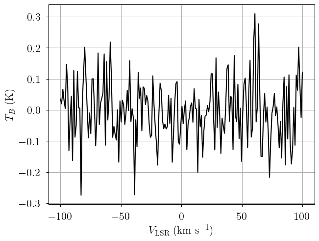
To test the model, we must simulate some data. We can do this with EmissionModel, but we must pack a “dummy” data structure first. The model expects the observation to be named "emission".

[2]:

from bayes_spec import SpecData

# spectral axes definition
velo_axis = np.linspace(-100.0, 100.0, 200) # km s-1

# data noise can either be a scalar (assumed constant noise across the spectrum)
# or an array of the same length as the data
rms = 0.1 # K

# brightness data. In this case, we just throw in some random data for now
# since we are only doing this in order to simulate some actual data.
emission = rms * np.random.randn(len(velo_axis))

dummy_data = {"emission": SpecData(
    velo_axis,
    emission,
    rms,
    xlabel=r"$V_{\rm LSR}$ (km s$^{-1}$)",
    ylabel=r"$T_B$ (K)",
)}

# Plot dummy data
fig, ax = plt.subplots(layout="constrained")
ax.plot(dummy_data["emission"].spectral, dummy_data["emission"].brightness, "k-")
ax.set_xlabel(dummy_data["emission"].xlabel)
_ = ax.set_ylabel(dummy_data["emission"].ylabel)

../_images/notebooks_emission_model_3_0.png

Now that we have a dummy data format, we can generate a simulated observation by evaluating the model. First we create the model.

[3]:

from caribou_hi import EmissionModel

# Initialize and define the model
n_clouds = 3
baseline_degree = 0
model = EmissionModel(
    dummy_data,
    n_clouds=n_clouds,
    baseline_degree=baseline_degree,
    bg_temp = 3.77, # assumed background temperature (K)
    seed=1234,
    verbose=True
)
model.add_priors(
    prior_filling_factor=[2.0, 1.0],  # filling factor prior shape
    prior_TB_fwhm=200.0, # peak brightness temperature x FWHM prior width (K km s-1)
    prior_tkin_factor=[2.0, 2.0], # kinetic temperature prior shape
    prior_fwhm2=200.0, # FWHM^2 prior width (km2 s-2)
    prior_log10_nHI=[0.0, 1.5],  # log10(density) prior mean and width (cm-3)
    prior_velocity=[-20.0, 20.0],  # lower and upper limit of velocity prior (km/s)
    prior_log10_n_alpha=[-6.0, 1.0],  # log10(n_alpha) prior width (cm-3)
    prior_fwhm_L=None,  # Assume Gaussian line profile
    prior_baseline_coeffs=None,  # Default baseline priors
)
model.add_likelihood()

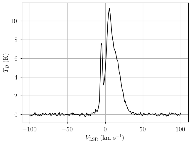
Now we simulate with a given set of simulation parameters.

[4]:

from caribou_hi import physics

# Simulation parameters
filling_factor = np.array([0.2, 0.8, 1.0])
log10_nHI = np.array([1.25, 0.0, -0.5])
tkin = np.array([50.0, 300.0, 5000.0])
log10_n_alpha = np.array([-5.5, -6.0, -6.5])
depth = np.array([5.0, 25.0, 300.0])
nth_fwhm_1pc = np.array([1.25, 1.75, 1.5])
depth_nth_fwhm_power = np.array([0.2, 0.3, 0.4])

tspin = physics.calc_spin_temp(tkin, 10.0**log10_nHI, 10.0**log10_n_alpha).eval()
print("tspin", tspin)

fwhm_nonthermal = physics.calc_nonthermal_fwhm(depth, nth_fwhm_1pc, depth_nth_fwhm_power)
fwhm2_thermal = physics.calc_thermal_fwhm2(tkin)
fwhm = np.sqrt(fwhm_nonthermal**2.0 + fwhm2_thermal)
print("fwhm", fwhm)

log10_Pth = np.log10(tkin) + log10_nHI
print("log10_Pth", log10_Pth)

log10_NHI = log10_nHI + np.log10(depth) + 18.489351
print("log10_NHI", log10_NHI)

tau_total = physics.calc_tau_total(10.0**log10_NHI, tspin)
print("tau_total", tau_total)

const = np.sqrt(2.0 * np.pi) / (2.0 * np.sqrt(2.0 * np.log(2.0)))
tau_peak = tau_total / fwhm / const
print("tau_peak", tau_peak)

TB_fwhm = filling_factor * tspin * (1.0 - np.exp(-tau_peak)) * fwhm
print("TB_fwhm", TB_fwhm)

sim_params = {
    "fwhm2": fwhm**2.0,
    "TB_fwhm": TB_fwhm,
    "tkin": tkin,
    "filling_factor": filling_factor,
    "log10_nHI": log10_nHI,
    "velocity": np.array([-5.0, 5.0, 10.0]),
    "log10_n_alpha": log10_n_alpha,
    "baseline_emission_norm": [0.0],
}

# add derived quantities to sim_params
for key in model.cloud_deterministics:
    if key not in sim_params.keys():
        sim_params[key] = model.model[key].eval(sim_params, on_unused_input="ignore")

# Evaluate and save simulated observation
emission = model.model["emission"].eval(sim_params, on_unused_input="ignore")
data = {"emission": SpecData(
    velo_axis,
    emission,
    rms,
    xlabel=r"$V_{\rm LSR}$ (km s$^{-1}$)",
    ylabel=r"$T_B$ (K)",
)}

tspin [  49.9920589   297.73994712 2795.52422645]
fwhm [ 2.29393108  5.90364916 21.08270953]
log10_Pth [2.94897    2.47712125 3.19897   ]
log10_NHI [20.438321   19.88729101 20.46647225]
tau_total [3.01140471 0.14216839 0.05745901]
tau_peak [1.23326541 0.02262301 0.00256035]
TB_fwhm [ 16.25359747  31.45536056 150.70696853]

[5]:

sim_params

[5]:

{'fwhm2': array([  5.26211978,  34.85307344, 444.48064099]),
 'TB_fwhm': array([ 16.25359747,  31.45536056, 150.70696853]),
 'tkin': array([  50.,  300., 5000.]),
 'filling_factor': array([0.2, 0.8, 1. ]),
 'log10_nHI': array([ 1.25,  0.  , -0.5 ]),
 'velocity': array([-5.,  5., 10.]),
 'log10_n_alpha': array([-5.5, -6. , -6.5]),
 'baseline_emission_norm': [0.0],
 'tspin': array([  49.9920589 ,  297.73994712, 2795.52422645]),
 'tau_total': array([3.01140471, 0.14216839, 0.05745901]),
 'log10_Pth': array([2.94897   , 2.47712125, 3.19897   ]),
 'log10_NHI': array([20.438321  , 19.88729101, 20.46647225]),
 'log10_depth': array([0.69897   , 1.39794001, 2.47712125])}

[6]:

# Plot data
fig, ax = plt.subplots(layout="constrained")
ax.plot(data["emission"].spectral, data["emission"].brightness, "k-")
ax.set_xlabel(data["emission"].xlabel)
_ = ax.set_ylabel(data["emission"].ylabel)

../_images/notebooks_emission_model_9_0.png

Model Definition

Finally, with our model definition and (simulated) data in hand, we can explore the capabilities of EmissionModel.

[7]:

# Initialize and define the model
model = EmissionModel(
    data,
    n_clouds=n_clouds,
    baseline_degree=baseline_degree,
    bg_temp = 3.77, # assumed background temperature (K)
    seed=1234,
    verbose=True
)
model.add_priors(
    prior_filling_factor=[2.0, 1.0],  # filling factor prior shape
    prior_TB_fwhm=200.0, # peak brightness temperature x FWHM prior width (K km s-1)
    prior_tkin_factor=[2.0, 2.0], # kinetic temperature prior shape
    prior_fwhm2=200.0, # FWHM^2 prior width (km2 s-2)
    prior_log10_nHI=[0.0, 1.5],  # log10(density) prior mean and width (cm-3)
    prior_velocity=[-20.0, 20.0],  # lower and upper limit of velocity prior (km/s)
    prior_log10_n_alpha=[-6.0, 1.0],  # log10(n_alpha) prior width (cm-3)
    prior_fwhm_L=None,  # Assume Gaussian line profile
    prior_baseline_coeffs=None,  # Default baseline priors
)
model.add_likelihood()

[8]:

# Plot model graph
model.graph().render('emission_model', format='png')
model.graph()

[8]:

../_images/notebooks_emission_model_12_0.svg

[9]:

# model string representation
print(model.model.str_repr())

baseline_emission_norm ~ Normal(0, 1)
            fwhm2_norm ~ Gamma(0.5, f())
        log10_nHI_norm ~ Normal(0, 1)
         velocity_norm ~ Beta(2, 2)
    log10_n_alpha_norm ~ Normal(0, 1)
          TB_fwhm_norm ~ HalfNormal(0, 1)
      tkin_factor_norm ~ Beta(2, 2)
        filling_factor ~ Beta(2, 1)
                 fwhm2 ~ Deterministic(f(fwhm2_norm))
             log10_nHI ~ Deterministic(f(log10_nHI_norm))
              velocity ~ Deterministic(f(velocity_norm))
         log10_n_alpha ~ Deterministic(f(log10_n_alpha_norm))
               TB_fwhm ~ Deterministic(f(TB_fwhm_norm))
                  tkin ~ Deterministic(f(tkin_factor_norm, fwhm2_norm, TB_fwhm_norm))
                 tspin ~ Deterministic(f(tkin_factor_norm, log10_n_alpha_norm, fwhm2_norm, TB_fwhm_norm, log10_nHI_norm))
             tau_total ~ Deterministic(f(fwhm2_norm, filling_factor, TB_fwhm_norm, tkin_factor_norm, log10_n_alpha_norm, log10_nHI_norm))
             log10_Pth ~ Deterministic(f(log10_nHI_norm, tkin_factor_norm, fwhm2_norm, TB_fwhm_norm))
             log10_NHI ~ Deterministic(f(fwhm2_norm, filling_factor, tkin_factor_norm, log10_n_alpha_norm, TB_fwhm_norm, log10_nHI_norm))
           log10_depth ~ Deterministic(f(log10_nHI_norm, fwhm2_norm, filling_factor, tkin_factor_norm, log10_n_alpha_norm, TB_fwhm_norm))
              emission ~ Normal(f(filling_factor, baseline_emission_norm, tkin_factor_norm, fwhm2_norm, log10_n_alpha_norm, TB_fwhm_norm, log10_nHI_norm, velocity_norm), <constant>)

We check that our prior distributions are reasonable by drawing prior predictive checks. Each colored line is a simulated “observation” with parameters drawn from the prior distributions. You should check that these simulated observations at least somewhat overlap your actual observation (black line).

[10]:

from bayes_spec.plots import plot_predictive

# prior predictive check
prior = model.sample_prior_predictive(
    samples=1000,  # prior predictive samples
)
_ = plot_predictive(model.data, prior.prior_predictive.sel(draw=slice(None, None, 20)))

Sampling: [TB_fwhm_norm, baseline_emission_norm, emission, filling_factor, fwhm2_norm, log10_nHI_norm, log10_n_alpha_norm, tkin_factor_norm, velocity_norm]

../_images/notebooks_emission_model_15_1.png

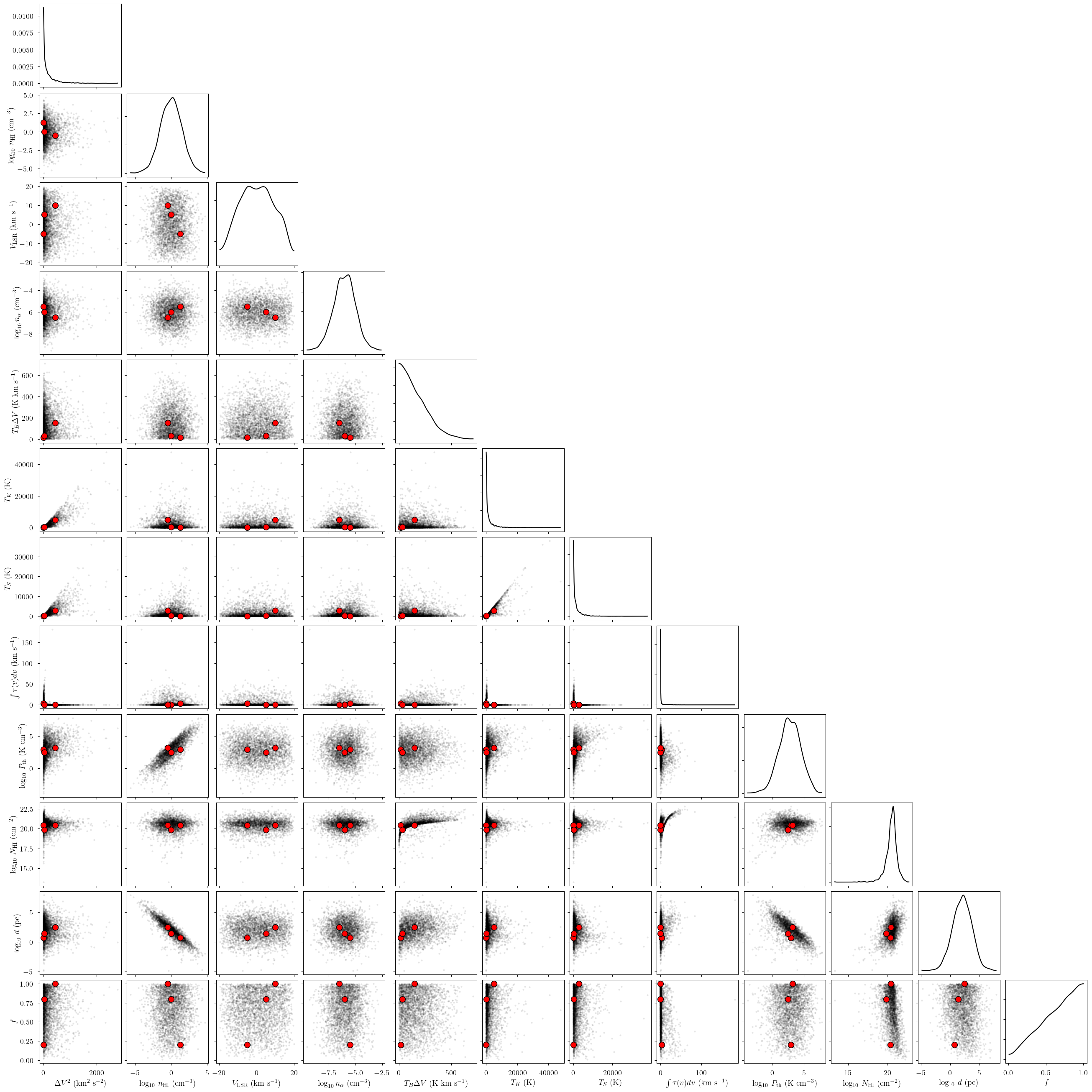
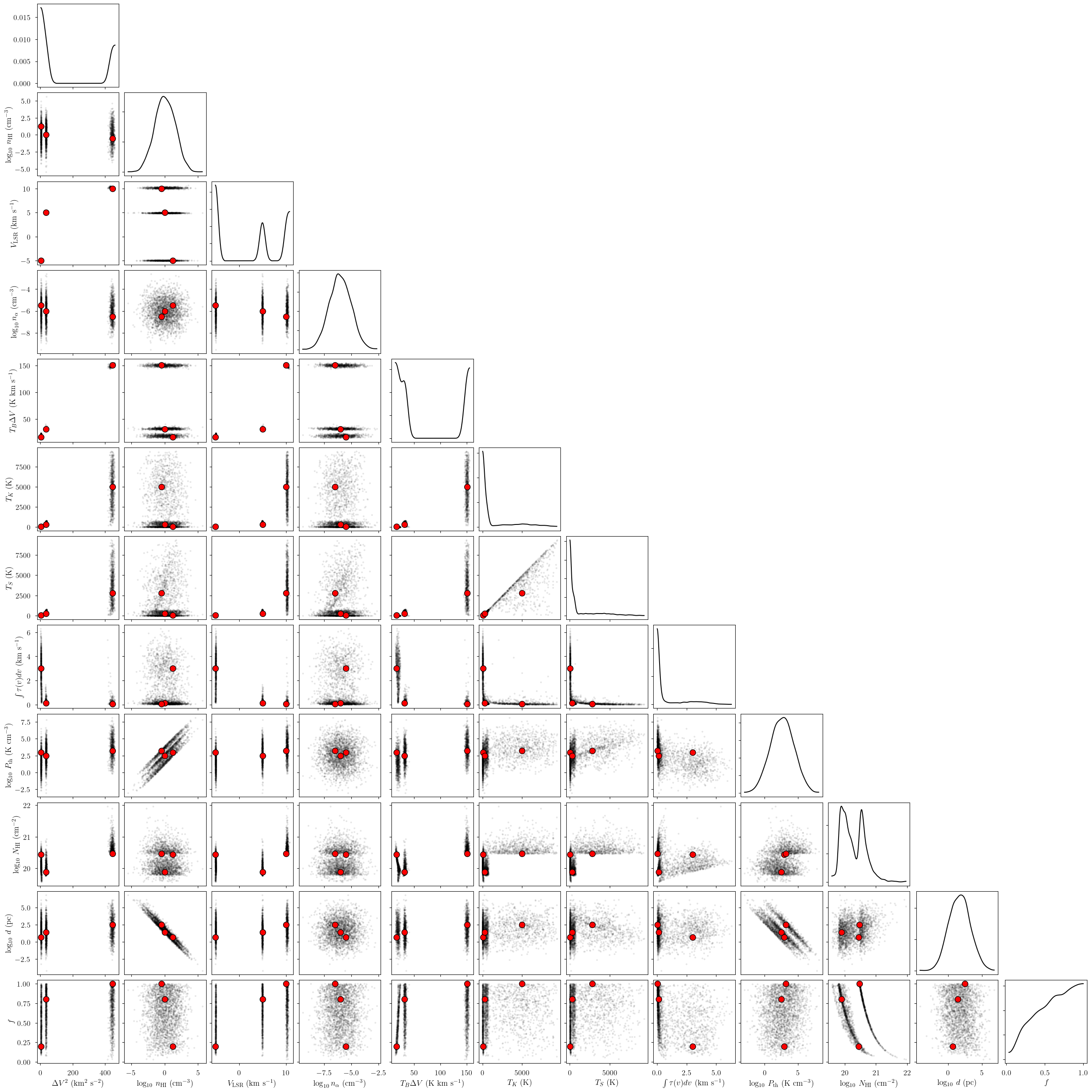
We can also check out our prior distributions impact the deterministic (derived) quantities in our model. The red points represent the simulation parameters.

[11]:

print(model.cloud_freeRVs)
print(model.cloud_deterministics)

['fwhm2_norm', 'log10_nHI_norm', 'velocity_norm', 'log10_n_alpha_norm', 'TB_fwhm_norm', 'tkin_factor_norm', 'filling_factor']
['fwhm2', 'log10_nHI', 'velocity', 'log10_n_alpha', 'TB_fwhm', 'tkin', 'tspin', 'tau_total', 'log10_Pth', 'log10_NHI', 'log10_depth']

[12]:

from bayes_spec.plots import plot_pair

var_names = model.cloud_deterministics + [p for p in model.cloud_freeRVs if "_norm" not in p]
print(var_names)
_ = plot_pair(
    prior.prior, # samples
    var_names, # var_names to plot
    combine_dims=["cloud"], # concatenate clouds
    labeller=model.labeller, # label manager
    kind="scatter", # plot type
    reference_values=sim_params, # truths
)

['fwhm2', 'log10_nHI', 'velocity', 'log10_n_alpha', 'TB_fwhm', 'tkin', 'tspin', 'tau_total', 'log10_Pth', 'log10_NHI', 'log10_depth', 'filling_factor']

../_images/notebooks_emission_model_18_1.png

Variational Inference

We can approximate the posterior distribution using variational inference.

[13]:

start = time.time()
model.fit(
    n = 1_000_000, # maximum number of VI iterations
    draws = 1_000, # number of posterior samples
    rel_tolerance = 0.005, # VI relative convergence threshold
    abs_tolerance = 0.005, # VI absolute convergence threshold
    learning_rate = 0.001, # VI learning rate
    start = {"velocity_norm": np.linspace(0.1, 0.9, n_clouds)},
)
end = time.time()
print(f"Runtime: {(end-start)/60.0:.2f} minutes")

Convergence achieved at 61600
Interrupted at 61,599 [6%]: Average Loss = 15,154

Adding log-likelihood to trace

Runtime: 0.87 minutes

[14]:

pm.summary(model.trace.posterior)

arviz - WARNING - Shape validation failed: input_shape: (1, 1000), minimum_shape: (chains=2, draws=4)

[14]:

	mean	sd	hdi_3%	hdi_97%	mcse_mean	mcse_sd	ess_bulk	ess_tail	r_hat
baseline_emission_norm[0]	0.013	0.071	-0.114	0.145	0.002	0.001	918.0	975.0	NaN
log10_nHI_norm[0]	0.058	1.004	-1.790	2.057	0.034	0.022	867.0	847.0	NaN
log10_nHI_norm[1]	0.065	0.974	-1.617	2.014	0.033	0.022	883.0	612.0	NaN
log10_nHI_norm[2]	0.085	0.923	-1.584	1.896	0.030	0.022	928.0	983.0	NaN
log10_n_alpha_norm[0]	-0.015	0.999	-2.093	1.686	0.034	0.024	880.0	1019.0	NaN
log10_n_alpha_norm[1]	0.070	0.990	-1.865	1.875	0.033	0.021	889.0	983.0	NaN
log10_n_alpha_norm[2]	0.065	0.969	-1.733	1.831	0.030	0.020	1037.0	983.0	NaN
fwhm2_norm[0]	0.034	0.001	0.032	0.036	0.000	0.000	1049.0	908.0	NaN
fwhm2_norm[1]	0.184	0.004	0.177	0.192	0.000	0.000	1002.0	900.0	NaN
fwhm2_norm[2]	2.188	0.019	2.152	2.224	0.001	0.000	938.0	909.0	NaN
velocity_norm[0]	0.375	0.000	0.374	0.376	0.000	0.000	1017.0	944.0	NaN
velocity_norm[1]	0.623	0.001	0.621	0.624	0.000	0.000	1065.0	908.0	NaN
velocity_norm[2]	0.756	0.001	0.754	0.758	0.000	0.000	901.0	908.0	NaN
TB_fwhm_norm[0]	0.094	0.001	0.092	0.096	0.000	0.000	976.0	941.0	NaN
TB_fwhm_norm[1]	0.163	0.001	0.160	0.165	0.000	0.000	887.0	985.0	NaN
TB_fwhm_norm[2]	0.745	0.003	0.740	0.750	0.000	0.000	1063.0	872.0	NaN
tkin_factor_norm[0]	0.650	0.114	0.436	0.856	0.004	0.002	1025.0	1023.0	NaN
tkin_factor_norm[1]	0.618	0.153	0.349	0.897	0.005	0.003	958.0	850.0	NaN
tkin_factor_norm[2]	0.509	0.220	0.132	0.890	0.007	0.004	943.0	796.0	NaN
filling_factor[0]	0.734	0.174	0.404	0.990	0.005	0.004	1049.0	1033.0	NaN
filling_factor[1]	0.692	0.222	0.287	0.993	0.007	0.005	864.0	941.0	NaN
filling_factor[2]	0.672	0.241	0.211	0.999	0.008	0.005	899.0	900.0	NaN
fwhm2[0]	6.833	0.198	6.471	7.218	0.006	0.005	1049.0	908.0	NaN
fwhm2[1]	36.826	0.821	35.321	38.378	0.026	0.019	1002.0	900.0	NaN
fwhm2[2]	437.689	3.884	430.387	444.782	0.127	0.094	938.0	909.0	NaN
log10_nHI[0]	0.087	1.506	-2.685	3.086	0.051	0.034	867.0	847.0	NaN
log10_nHI[1]	0.098	1.461	-2.426	3.021	0.049	0.033	883.0	612.0	NaN
log10_nHI[2]	0.127	1.384	-2.376	2.843	0.045	0.033	928.0	983.0	NaN
velocity[0]	-4.996	0.017	-5.031	-4.967	0.001	0.000	1017.0	944.0	NaN
velocity[1]	4.910	0.034	4.845	4.971	0.001	0.001	1065.0	908.0	NaN
velocity[2]	10.256	0.045	10.170	10.340	0.002	0.001	901.0	908.0	NaN
log10_n_alpha[0]	-6.015	0.999	-8.093	-4.314	0.034	0.024	880.0	1019.0	NaN
log10_n_alpha[1]	-5.930	0.990	-7.865	-4.125	0.033	0.021	889.0	983.0	NaN
log10_n_alpha[2]	-5.935	0.969	-7.733	-4.169	0.030	0.020	1037.0	983.0	NaN
TB_fwhm[0]	18.812	0.207	18.435	19.199	0.007	0.005	976.0	941.0	NaN
TB_fwhm[1]	32.577	0.294	31.969	33.085	0.010	0.007	887.0	985.0	NaN
TB_fwhm[2]	149.094	0.541	147.973	150.024	0.017	0.012	1063.0	872.0	NaN
tkin[0]	99.564	16.378	68.569	128.293	0.510	0.349	1035.0	882.0	NaN
tkin[1]	499.610	122.735	273.370	719.607	3.941	2.651	971.0	841.0	NaN
tkin[2]	4871.837	2107.265	1318.416	8568.653	67.616	34.334	945.0	793.0	NaN
tspin[0]	98.995	16.324	67.978	128.070	0.523	0.343	1004.0	1020.0	NaN
tspin[1]	485.799	122.111	268.203	715.705	3.796	2.753	1035.0	947.0	NaN
tspin[2]	3933.974	1985.666	739.060	7567.764	60.423	33.959	1040.0	881.0	NaN
tau_total[0]	0.334	0.174	0.169	0.601	0.006	0.019	1075.0	978.0	NaN
tau_total[1]	0.146	0.187	0.053	0.305	0.006	0.038	810.0	972.0	NaN
tau_total[2]	0.127	0.291	0.020	0.327	0.009	0.092	930.0	843.0	NaN
log10_Pth[0]	2.079	1.512	-0.763	5.015	0.051	0.034	870.0	847.0	NaN
log10_Pth[1]	2.781	1.468	0.052	5.421	0.049	0.033	896.0	737.0	NaN
log10_Pth[2]	3.760	1.401	1.101	6.354	0.046	0.033	946.0	944.0	NaN
log10_NHI[0]	19.738	0.139	19.578	20.002	0.004	0.006	1005.0	1036.0	NaN
log10_NHI[1]	20.000	0.204	19.803	20.355	0.007	0.010	843.0	941.0	NaN
log10_NHI[2]	20.680	0.230	20.463	21.143	0.008	0.009	897.0	898.0	NaN
log10_depth[0]	1.162	1.510	-1.677	4.117	0.051	0.034	885.0	847.0	NaN
log10_depth[1]	1.413	1.483	-1.351	4.246	0.051	0.033	853.0	872.0	NaN
log10_depth[2]	2.063	1.399	-0.749	4.519	0.046	0.033	915.0	917.0	NaN

[15]:

posterior = model.sample_posterior_predictive(
    thin=10, # keep one in {thin} posterior samples
)
_ = plot_predictive(model.data, posterior.posterior_predictive)

Sampling: [emission]

../_images/notebooks_emission_model_22_3.png

Posterior Sampling: MCMC

We can sample from the posterior distribution using MCMC. We increase target_accept because this model has some degeneracies.

[16]:

start = time.time()
model.sample(
    init="advi+adapt_diag",  # initialization strategy
    tune=1000,  # tuning samples
    draws=1000,  # posterior samples
    chains=8,  # number of independent chains
    cores=8,  # number of parallel chains
    init_kwargs={
        "rel_tolerance": 0.005,
        "abs_tolerance": 0.005,
        "learning_rate": 0.001,
        "start": {"velocity_norm": np.linspace(0.1, 0.9, n_clouds)},
    },  # VI initialization arguments
    nuts_kwargs={"target_accept": 0.9},  # NUTS arguments
)
end = time.time()
print(f"Runtime: {(end-start)/60.0:.2f} minutes")

Initializing NUTS using custom advi+adapt_diag strategy

Convergence achieved at 61600
Interrupted at 61,599 [6%]: Average Loss = 15,154
Multiprocess sampling (8 chains in 8 jobs)
NUTS: [baseline_emission_norm, fwhm2_norm, log10_nHI_norm, velocity_norm, log10_n_alpha_norm, TB_fwhm_norm, tkin_factor_norm, filling_factor]

Sampling 8 chains for 1_000 tune and 1_000 draw iterations (8_000 + 8_000 draws total) took 58 seconds.

Adding log-likelihood to trace

There were 774 divergences in converged chains.
Runtime: 2.00 minutes

[17]:

model.solve(
    init_params="random_from_data", # GMM initialization strategy
    n_init=10, # number of GMM initilizations
    max_iter=1_000, # maximum number of GMM iterations
    kl_div_threshold=0.1, # covergence threshold
)

GMM converged to unique solution

Check that the effective sample sizes are large and the covergence statistic r_hat is close to 1! If not, you may have to increase the number of tuning steps (tune=2000) or the NUTS acceptance rate (target_accept=0.9).

[18]:

print("solutions:", model.solutions)
az.summary(model.trace["solution_0"])
# this also works: az.summary(model.trace.solution_0)

solutions: [0]

[18]:

	mean	sd	hdi_3%	hdi_97%	mcse_mean	mcse_sd	ess_bulk	ess_tail	r_hat
baseline_emission_norm[0]	0.006	0.080	-0.146	0.153	0.001	0.001	3689.0	3661.0	1.00
log10_nHI_norm[0]	0.005	0.989	-1.815	1.838	0.014	0.014	4675.0	3636.0	1.00
log10_nHI_norm[1]	0.013	1.016	-1.871	1.934	0.020	0.018	2694.0	993.0	1.00
log10_nHI_norm[2]	-0.006	1.006	-1.893	1.912	0.018	0.014	3244.0	2621.0	1.00
log10_n_alpha_norm[0]	-0.015	1.021	-1.883	1.924	0.016	0.013	3904.0	3853.0	1.00
log10_n_alpha_norm[1]	0.010	0.991	-1.871	1.813	0.015	0.013	4128.0	3608.0	1.00
log10_n_alpha_norm[2]	-0.020	0.992	-1.952	1.778	0.016	0.012	3761.0	3036.0	1.00
fwhm2_norm[0]	0.026	0.004	0.019	0.035	0.000	0.000	820.0	801.0	1.02
fwhm2_norm[1]	0.179	0.009	0.163	0.196	0.000	0.000	1586.0	1568.0	1.01
fwhm2_norm[2]	2.211	0.034	2.149	2.278	0.001	0.001	1507.0	1054.0	1.01
velocity_norm[0]	0.376	0.001	0.375	0.377	0.000	0.000	2434.0	4114.0	1.00
velocity_norm[1]	0.623	0.001	0.621	0.625	0.000	0.000	2452.0	3019.0	1.00
velocity_norm[2]	0.754	0.003	0.749	0.760	0.000	0.000	1144.0	1235.0	1.01
TB_fwhm_norm[0]	0.093	0.010	0.075	0.113	0.000	0.000	722.0	892.0	1.02
TB_fwhm_norm[1]	0.160	0.007	0.148	0.173	0.000	0.000	1245.0	1210.0	1.01
TB_fwhm_norm[2]	0.753	0.009	0.735	0.769	0.000	0.000	1117.0	1141.0	1.01
tkin_factor_norm[0]	0.259	0.195	0.020	0.644	0.005	0.003	1429.0	2694.0	1.00
tkin_factor_norm[1]	0.519	0.217	0.133	0.899	0.004	0.003	2654.0	2010.0	1.00
tkin_factor_norm[2]	0.499	0.221	0.093	0.881	0.003	0.002	4968.0	4229.0	1.00
filling_factor[0]	0.524	0.244	0.136	0.951	0.007	0.002	1175.0	1954.0	1.01
filling_factor[1]	0.681	0.225	0.288	1.000	0.004	0.002	3117.0	1691.0	1.00
filling_factor[2]	0.666	0.230	0.250	1.000	0.003	0.003	3755.0	2223.0	1.00
fwhm2[0]	5.179	0.855	3.867	6.954	0.029	0.013	820.0	801.0	1.02
fwhm2[1]	35.822	1.744	32.583	39.205	0.044	0.029	1586.0	1568.0	1.01
fwhm2[2]	442.253	6.899	429.898	455.610	0.177	0.114	1507.0	1054.0	1.01
log10_nHI[0]	0.007	1.483	-2.723	2.757	0.022	0.021	4675.0	3636.0	1.00
log10_nHI[1]	0.019	1.524	-2.807	2.901	0.030	0.027	2694.0	993.0	1.00
log10_nHI[2]	-0.009	1.509	-2.839	2.868	0.026	0.021	3244.0	2621.0	1.00
velocity[0]	-4.978	0.022	-5.020	-4.937	0.000	0.000	2434.0	4114.0	1.00
velocity[1]	4.936	0.042	4.856	5.012	0.001	0.001	2452.0	3019.0	1.00
velocity[2]	10.171	0.115	9.954	10.386	0.003	0.002	1144.0	1235.0	1.01
log10_n_alpha[0]	-6.015	1.021	-7.883	-4.076	0.016	0.013	3904.0	3853.0	1.00
log10_n_alpha[1]	-5.990	0.991	-7.871	-4.187	0.015	0.013	4128.0	3608.0	1.00
log10_n_alpha[2]	-6.020	0.992	-7.952	-4.222	0.016	0.012	3761.0	3036.0	1.00
TB_fwhm[0]	18.638	2.024	15.082	22.527	0.073	0.030	722.0	892.0	1.02
TB_fwhm[1]	32.062	1.364	29.660	34.568	0.038	0.042	1245.0	1210.0	1.01
TB_fwhm[2]	150.555	1.833	146.981	153.892	0.055	0.039	1117.0	1141.0	1.01
tkin[0]	37.132	24.263	12.396	85.315	0.594	0.476	1454.0	3128.0	1.00
tkin[1]	410.114	172.369	104.034	717.518	3.145	2.046	2828.0	1959.0	1.00
tkin[2]	4828.272	2137.886	952.054	8581.388	30.347	23.613	4988.0	4274.0	1.00
tspin[0]	36.989	24.095	12.268	84.833	0.589	0.471	1456.0	3139.0	1.00
tspin[1]	397.763	167.061	97.720	694.418	3.041	1.933	2824.0	2006.0	1.00
tspin[2]	3786.672	2069.101	147.597	7358.867	35.086	21.797	3148.0	2308.0	1.00
tau_total[0]	2.827	1.338	0.200	4.825	0.043	0.021	947.0	966.0	1.02
tau_total[1]	0.210	0.232	0.045	0.542	0.005	0.013	2907.0	2450.0	1.00
tau_total[2]	0.150	0.279	0.018	0.451	0.006	0.021	3085.0	3296.0	1.00
log10_Pth[0]	1.501	1.503	-1.259	4.339	0.023	0.021	4317.0	3804.0	1.00
log10_Pth[1]	2.581	1.537	-0.452	5.331	0.030	0.025	2755.0	1099.0	1.00
log10_Pth[2]	3.615	1.532	0.758	6.550	0.027	0.021	3304.0	2790.0	1.00
log10_NHI[0]	20.126	0.237	19.678	20.591	0.007	0.004	1019.0	1439.0	1.02
log10_NHI[1]	20.000	0.192	19.767	20.348	0.003	0.003	2686.0	1385.0	1.00
log10_NHI[2]	20.682	0.211	20.457	21.070	0.003	0.006	3921.0	3059.0	1.00
log10_depth[0]	1.629	1.500	-1.218	4.368	0.022	0.021	4563.0	3623.0	1.00
log10_depth[1]	1.492	1.533	-1.205	4.527	0.030	0.027	2660.0	1004.0	1.00
log10_depth[2]	2.202	1.535	-0.880	4.916	0.027	0.022	3122.0	2609.0	1.00

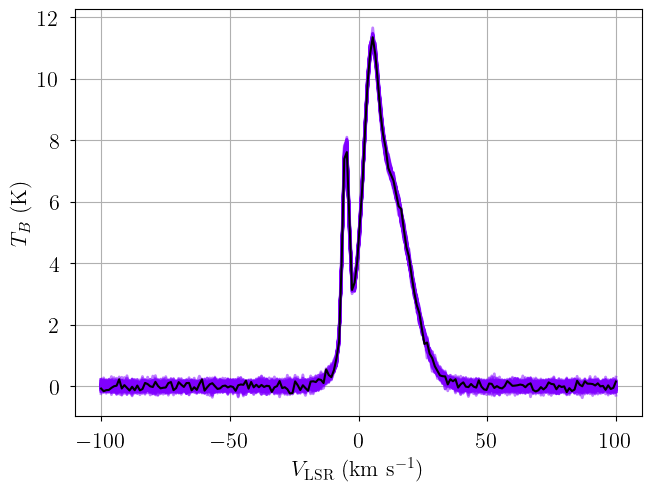
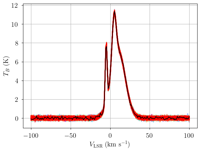
We generate posterior predictive checks as well as a trace plot of the individual chains. In the posterior predictive plot, we show each chain as a different color. Each line is one posterior sample.

[19]:

posterior = model.sample_posterior_predictive(
    thin=10, # keep one in {thin} posterior samples
)
_ = plot_predictive(model.data, posterior.posterior_predictive)

Sampling: [emission]

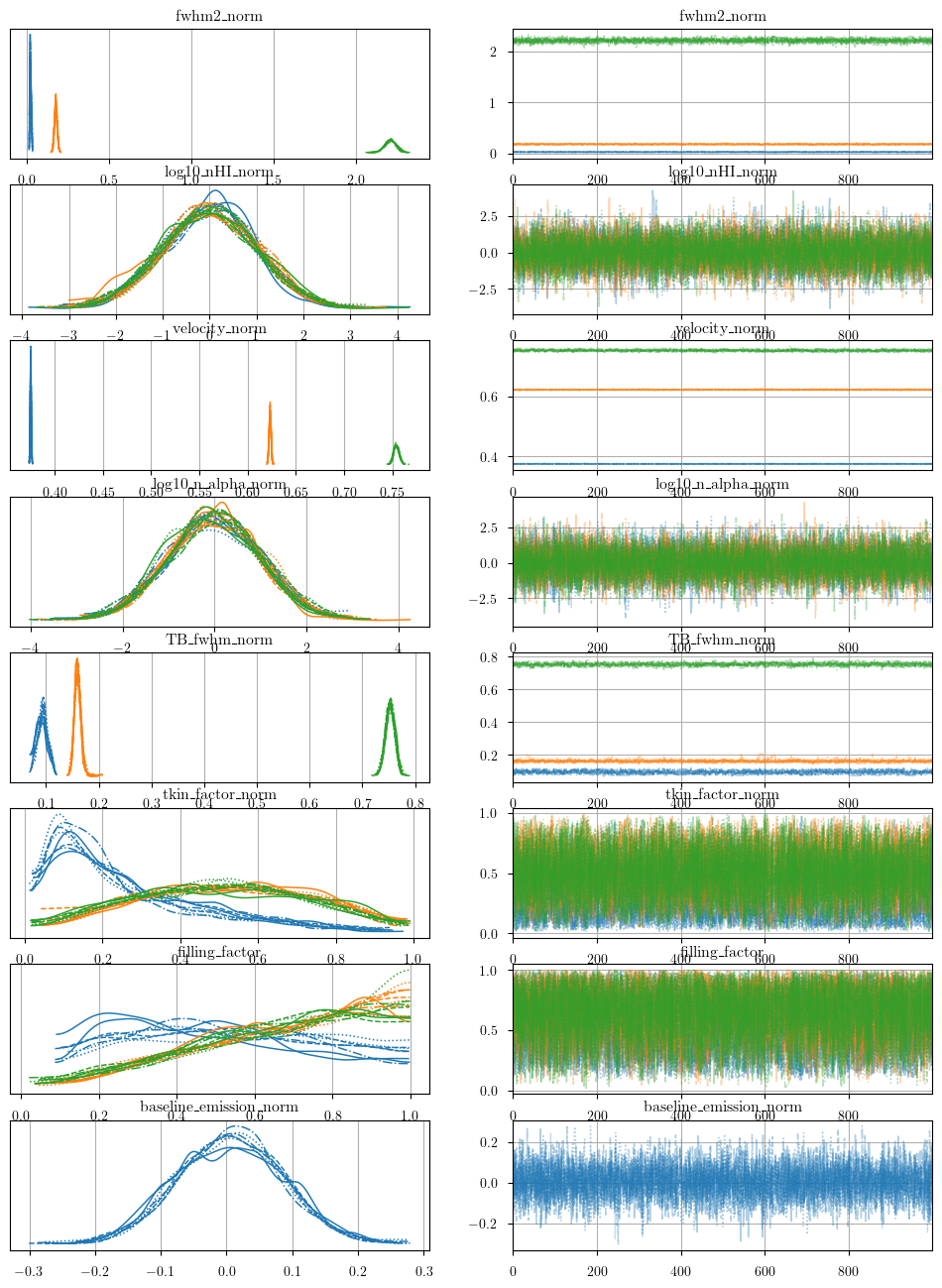
../_images/notebooks_emission_model_29_3.png

[20]:

from bayes_spec.plots import plot_traces

_ = plot_traces(model.trace.posterior, model.cloud_freeRVs + model.baseline_freeRVs + model.hyper_freeRVs)

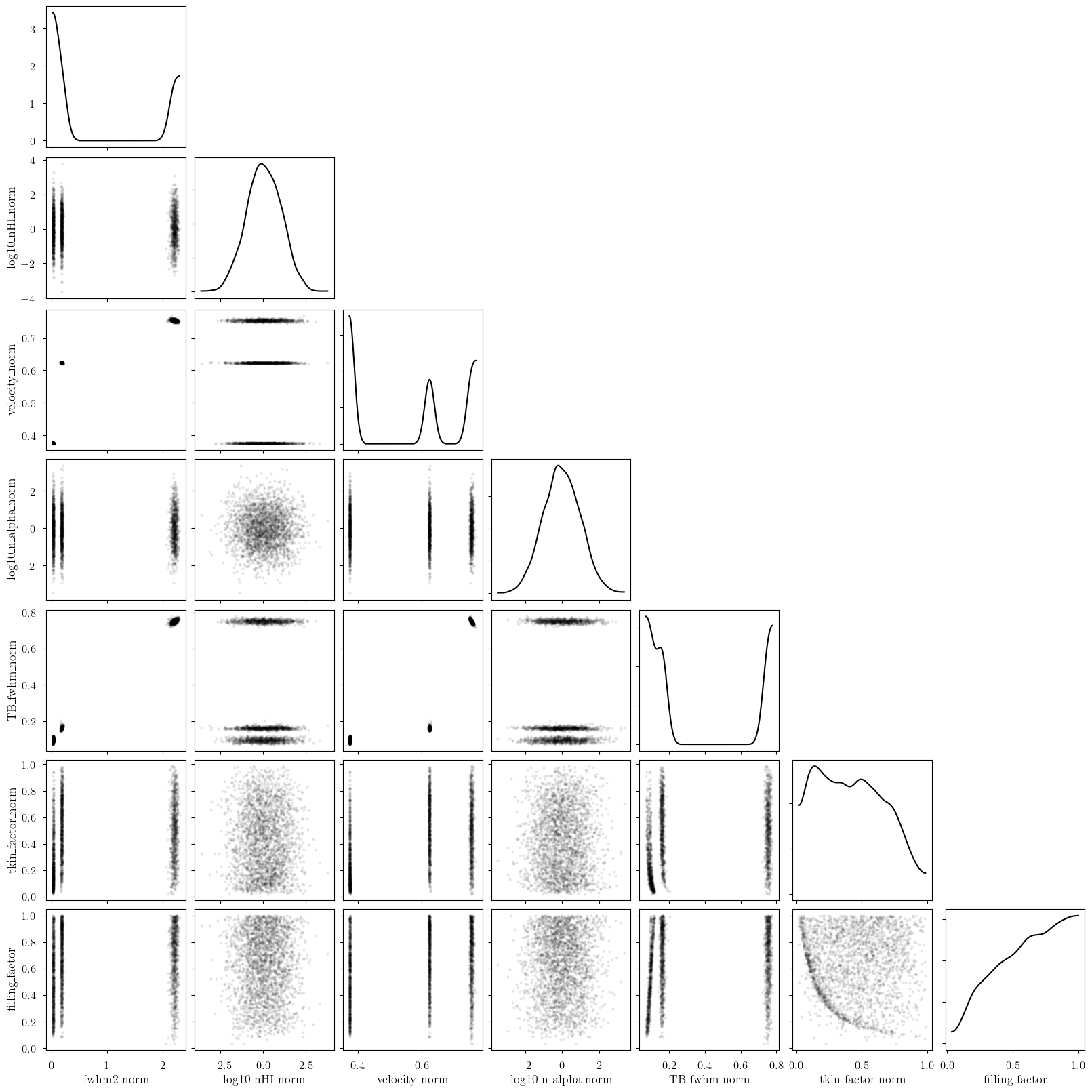
../_images/notebooks_emission_model_30_0.png

We can inspect the posterior distribution pair plots. First, the free parameters for all clouds. Keep an eye out for any strong degeneracies or non-linear correlations. If present, then these features can cause the posterior sampling to be inefficient. It may be worth re-parameterizing your model to remove these effects. Alternatively, increasing tune and target_accept can help.

[21]:

_ = plot_pair(
    model.trace.solution_0.sel(draw=slice(None, None, 10)), # samples
    model.cloud_freeRVs, # var_names to plot
    combine_dims=["cloud"], # concatenate clouds
    kind="scatter", # plot type
)

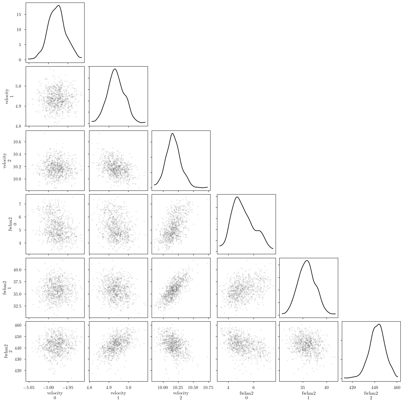
../_images/notebooks_emission_model_32_0.png

[22]:

_ = plot_pair(
    model.trace.solution_0.sel(draw=slice(None, None, 10)), # samples
    ["velocity", "fwhm2"], # var_names to plot
    combine_dims=None, # do not concatenate clouds
    kind="scatter", # plot type
)

../_images/notebooks_emission_model_33_0.png

[23]:

_ = plot_pair(
    model.trace.solution_0.sel(cloud=0, draw=slice(None, None, 10)), # samples
    model.cloud_freeRVs + model.hyper_freeRVs + model.baseline_freeRVs, # var_names to plot
    kind="scatter", # plot type
)

../_images/notebooks_emission_model_34_0.png

[24]:

_ = plot_pair(
    model.trace.solution_0.sel(cloud=1, draw=slice(None, None, 10)), # samples
    model.cloud_freeRVs + model.hyper_freeRVs + model.baseline_freeRVs, # var_names to plot
    kind="scatter", # plot type
)

../_images/notebooks_emission_model_35_0.png

[25]:

_ = plot_pair(
    model.trace.solution_0.sel(cloud=2, draw=slice(None, None, 10)), # samples
    model.cloud_freeRVs + model.hyper_freeRVs + model.baseline_freeRVs, # var_names to plot
    kind="scatter", # plot type
)

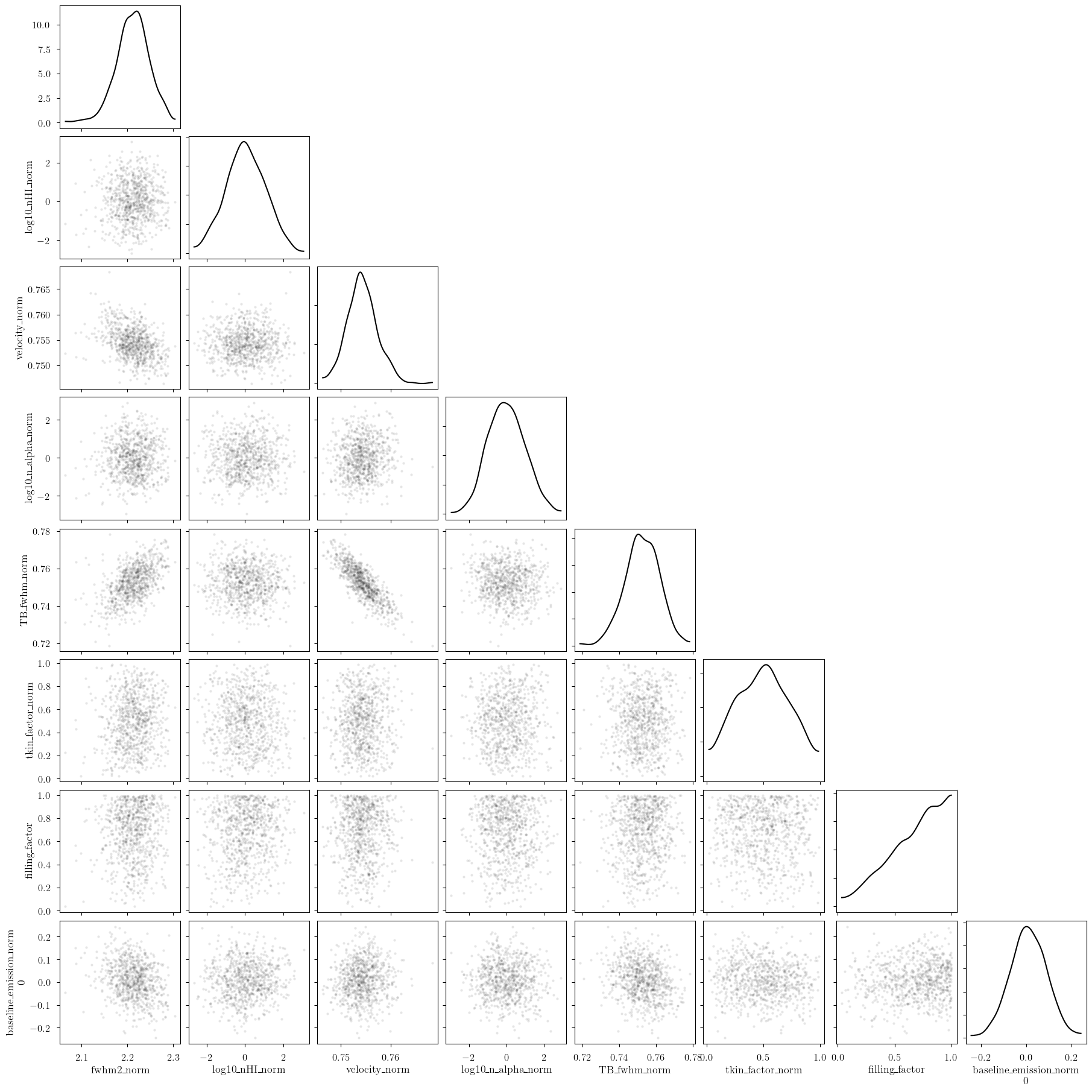
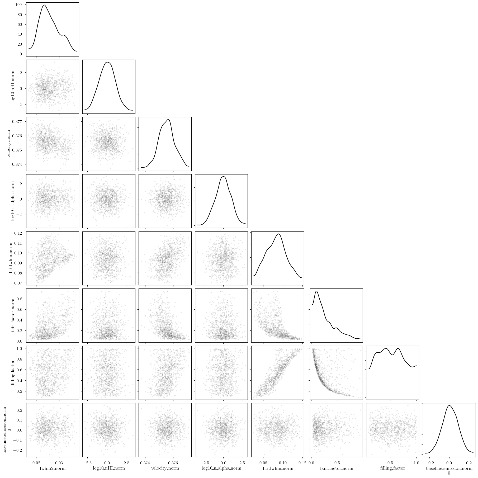
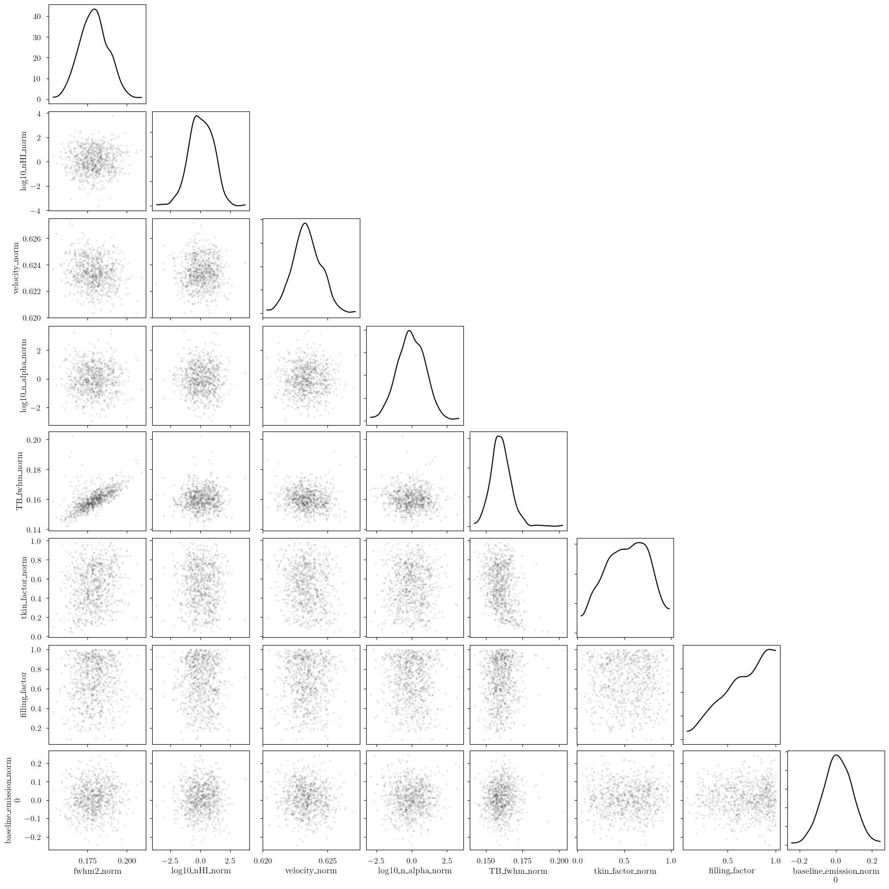
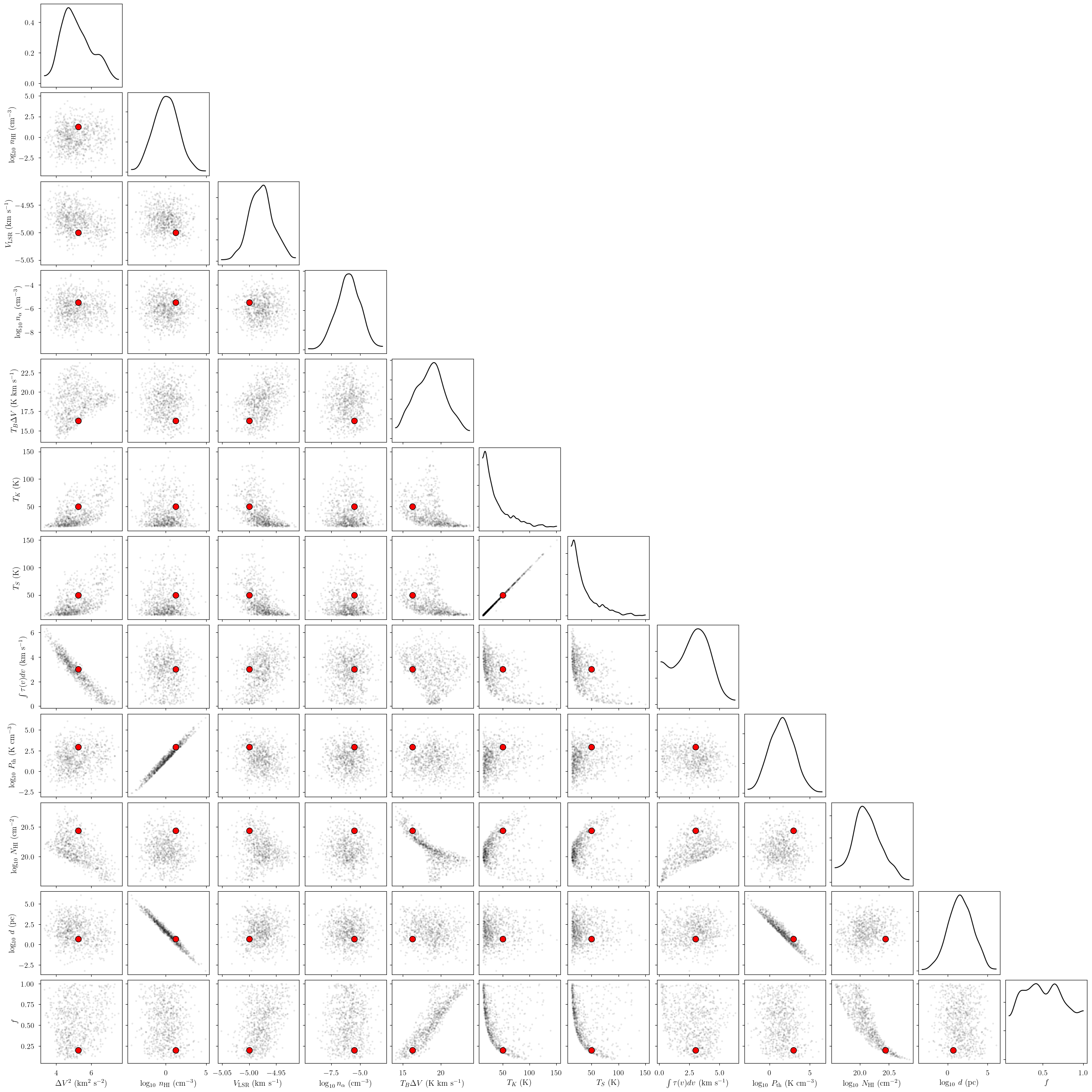
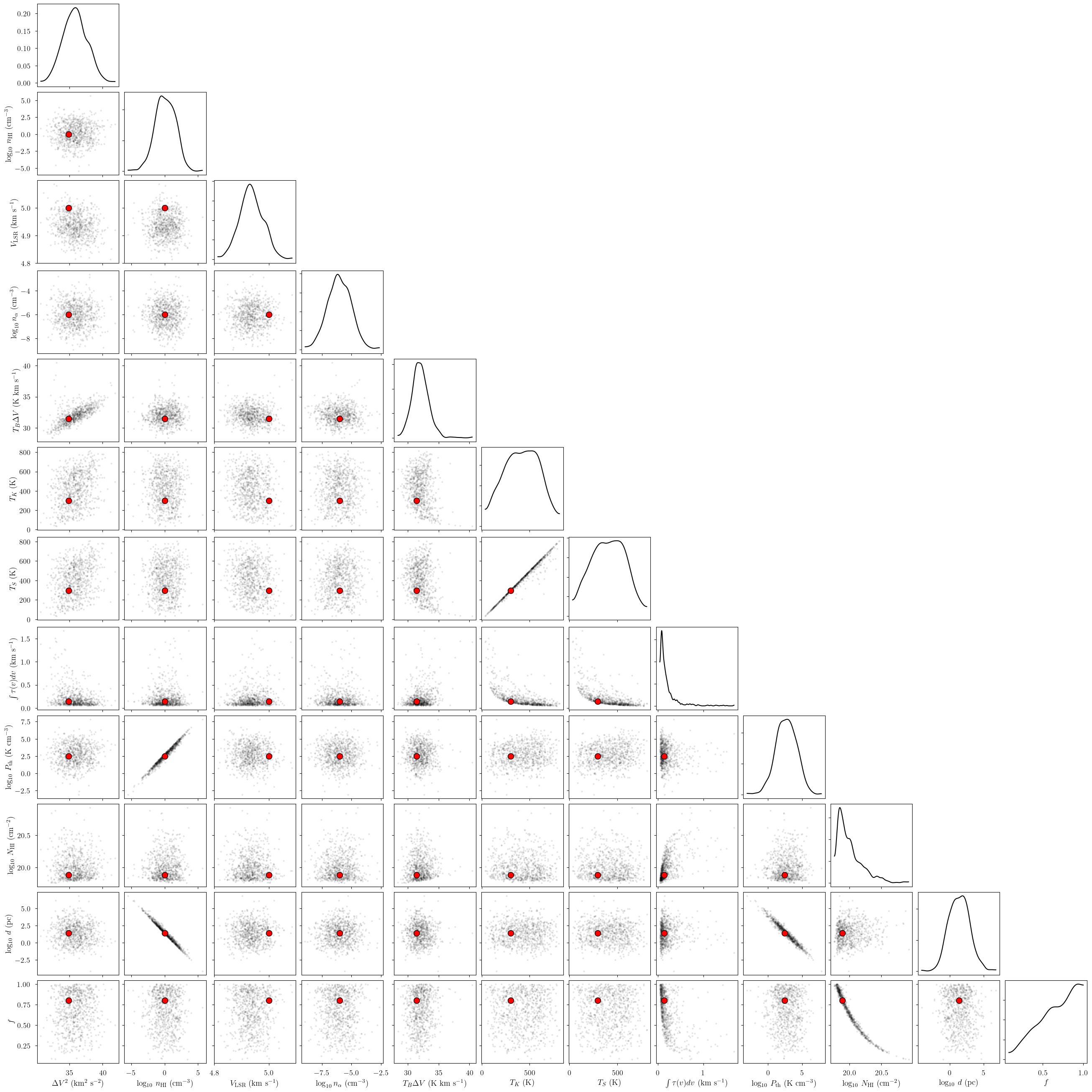
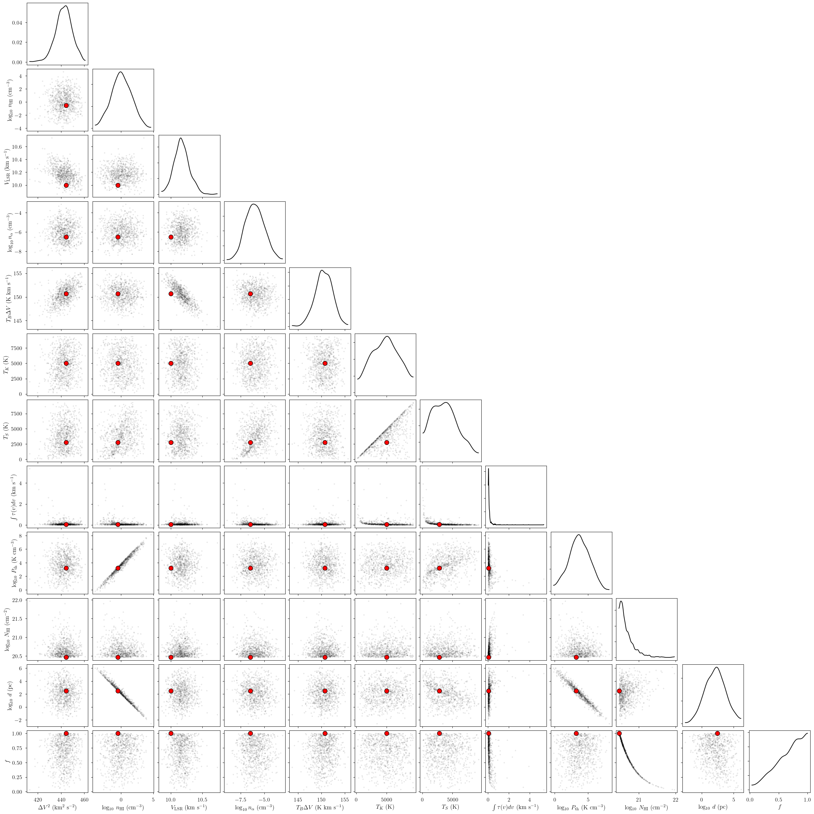
../_images/notebooks_emission_model_36_0.png

The red points represent the simulation parameters for the deterministic quantities.

[26]:

_ = plot_pair(
    model.trace.solution_0.sel(draw=slice(None, None, 10)), # samples
    var_names, # var_names to plot
    combine_dims=["cloud"], # concatenate clouds
    labeller=model.labeller, # label manager
    kind="scatter", # plot type
    reference_values=sim_params, # truths
)

../_images/notebooks_emission_model_38_0.png

[27]:

# identify simulation cloud corresponding to each posterior cloud
sim_cloud_map = {}
for i in range(n_clouds):
    posterior_velocity = model.trace.solution_0['velocity'].sel(cloud=i).data.mean()
    match = np.argmin(np.abs(sim_params["velocity"] - posterior_velocity))
    sim_cloud_map[i] = match
sim_cloud_map

[27]:

{0: np.int64(0), 1: np.int64(1), 2: np.int64(2)}

[28]:

print("cloud freeRVs", model.cloud_freeRVs)
print("cloud deterministics", model.cloud_deterministics)
print("hyper freeRVs", model.hyper_freeRVs)
print("hyper deterministics", model.hyper_deterministics)

cloud freeRVs ['fwhm2_norm', 'log10_nHI_norm', 'velocity_norm', 'log10_n_alpha_norm', 'TB_fwhm_norm', 'tkin_factor_norm', 'filling_factor']
cloud deterministics ['fwhm2', 'log10_nHI', 'velocity', 'log10_n_alpha', 'TB_fwhm', 'tkin', 'tspin', 'tau_total', 'log10_Pth', 'log10_NHI', 'log10_depth']
hyper freeRVs []
hyper deterministics []

[29]:

cloud = 0

# subset of sim_params
my_sim_params = {}
for var_name in var_names:
    my_sim_params[var_name] = sim_params[var_name][sim_cloud_map[cloud]]

_ = plot_pair(
    model.trace.solution_0.sel(cloud=cloud, draw=slice(None, None, 10)), # samples
    var_names, # var_names to plot
    labeller=model.labeller, # label manager
    kind="scatter", # plot type
    reference_values=my_sim_params, # truths
)

../_images/notebooks_emission_model_41_0.png

[30]:

cloud = 1

# subset of sim_params
my_sim_params = {}
for var_name in var_names:
    my_sim_params[var_name] = sim_params[var_name][sim_cloud_map[cloud]]

_ = plot_pair(
    model.trace.solution_0.sel(cloud=cloud, draw=slice(None, None, 10)), # samples
    var_names, # var_names to plot
    labeller=model.labeller, # label manager
    kind="scatter", # plot type
    reference_values=my_sim_params, # truths
)

../_images/notebooks_emission_model_42_0.png

[31]:

cloud = 2

# subset of sim_params
my_sim_params = {}
for var_name in var_names:
    my_sim_params[var_name] = sim_params[var_name][sim_cloud_map[cloud]]

_ = plot_pair(
    model.trace.solution_0.sel(cloud=cloud, draw=slice(None, None, 10)), # samples
    var_names, # var_names to plot
    labeller=model.labeller, # label manager
    kind="scatter", # plot type
    reference_values=my_sim_params, # truths
)

../_images/notebooks_emission_model_43_0.png

Finally, we can get the posterior statistics, Bayesian Information Criterion (BIC), etc.

[32]:

point_stats = az.summary(model.trace.solution_0, kind='stats')
print("BIC:", model.bic())
display(point_stats)

BIC: -237.1501253338259

	mean	sd	hdi_3%	hdi_97%
baseline_emission_norm[0]	0.006	0.080	-0.146	0.153
log10_nHI_norm[0]	0.005	0.989	-1.815	1.838
log10_nHI_norm[1]	0.013	1.016	-1.871	1.934
log10_nHI_norm[2]	-0.006	1.006	-1.893	1.912
log10_n_alpha_norm[0]	-0.015	1.021	-1.883	1.924
log10_n_alpha_norm[1]	0.010	0.991	-1.871	1.813
log10_n_alpha_norm[2]	-0.020	0.992	-1.952	1.778
fwhm2_norm[0]	0.026	0.004	0.019	0.035
fwhm2_norm[1]	0.179	0.009	0.163	0.196
fwhm2_norm[2]	2.211	0.034	2.149	2.278
velocity_norm[0]	0.376	0.001	0.375	0.377
velocity_norm[1]	0.623	0.001	0.621	0.625
velocity_norm[2]	0.754	0.003	0.749	0.760
TB_fwhm_norm[0]	0.093	0.010	0.075	0.113
TB_fwhm_norm[1]	0.160	0.007	0.148	0.173
TB_fwhm_norm[2]	0.753	0.009	0.735	0.769
tkin_factor_norm[0]	0.259	0.195	0.020	0.644
tkin_factor_norm[1]	0.519	0.217	0.133	0.899
tkin_factor_norm[2]	0.499	0.221	0.093	0.881
filling_factor[0]	0.524	0.244	0.136	0.951
filling_factor[1]	0.681	0.225	0.288	1.000
filling_factor[2]	0.666	0.230	0.250	1.000
fwhm2[0]	5.179	0.855	3.867	6.954
fwhm2[1]	35.822	1.744	32.583	39.205
fwhm2[2]	442.253	6.899	429.898	455.610
log10_nHI[0]	0.007	1.483	-2.723	2.757
log10_nHI[1]	0.019	1.524	-2.807	2.901
log10_nHI[2]	-0.009	1.509	-2.839	2.868
velocity[0]	-4.978	0.022	-5.020	-4.937
velocity[1]	4.936	0.042	4.856	5.012
velocity[2]	10.171	0.115	9.954	10.386
log10_n_alpha[0]	-6.015	1.021	-7.883	-4.076
log10_n_alpha[1]	-5.990	0.991	-7.871	-4.187
log10_n_alpha[2]	-6.020	0.992	-7.952	-4.222
TB_fwhm[0]	18.638	2.024	15.082	22.527
TB_fwhm[1]	32.062	1.364	29.660	34.568
TB_fwhm[2]	150.555	1.833	146.981	153.892
tkin[0]	37.132	24.263	12.396	85.315
tkin[1]	410.114	172.369	104.034	717.518
tkin[2]	4828.272	2137.886	952.054	8581.388
tspin[0]	36.989	24.095	12.268	84.833
tspin[1]	397.763	167.061	97.720	694.418
tspin[2]	3786.672	2069.101	147.597	7358.867
tau_total[0]	2.827	1.338	0.200	4.825
tau_total[1]	0.210	0.232	0.045	0.542
tau_total[2]	0.150	0.279	0.018	0.451
log10_Pth[0]	1.501	1.503	-1.259	4.339
log10_Pth[1]	2.581	1.537	-0.452	5.331
log10_Pth[2]	3.615	1.532	0.758	6.550
log10_NHI[0]	20.126	0.237	19.678	20.591
log10_NHI[1]	20.000	0.192	19.767	20.348
log10_NHI[2]	20.682	0.211	20.457	21.070
log10_depth[0]	1.629	1.500	-1.218	4.368
log10_depth[1]	1.492	1.533	-1.205	4.527
log10_depth[2]	2.202	1.535	-0.880	4.916

[ ]:

EmissionModel Tutorial

Simulating Data

Model Definition

Variational Inference

Posterior Sampling: MCMC

`EmissionModel` Tutorial