EmissionAbsorptionModel Tutorial
Trey V. Wenger (c) July 2025
Here we demonstrate the basic features of the EmissionAbsorptionModel model. EmissionAbsorptionModel models both 21cm emission and absorption observations simultaneously.
[1]:
# General imports
import time

import matplotlib.pyplot as plt
import arviz as az
import pandas as pd
import numpy as np
import pymc as pm

print("pymc version:", pm.__version__)
print("arviz version:", az.__version__)

import bayes_spec
print("bayes_spec version:", bayes_spec.__version__)

import caribou_hi
print("caribou_hi version:", caribou_hi.__version__)

# Notebook configuration
pd.options.display.max_rows = None
pymc version: 5.22.0
arviz version: 0.22.0dev
bayes_spec version: 1.9.0
caribou_hi version: 4.1.0+3.g94a913e.dirty
Simulating Data
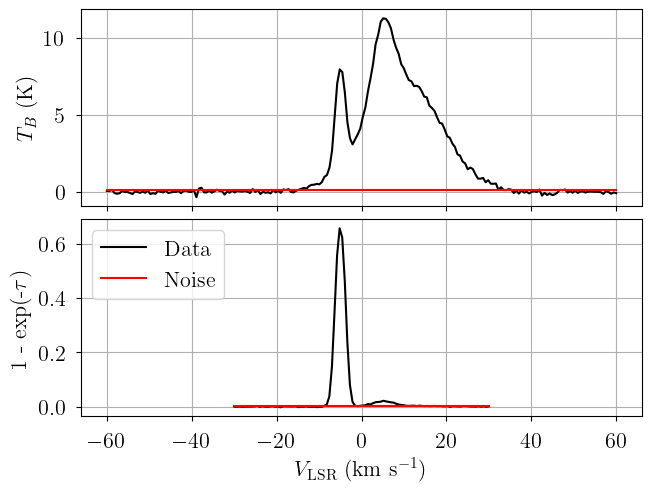
To test the model, we must simulate some data. We can do this with EmissionAbsorptionModel, but we must pack a “dummy” data structure first. The model expects the observations to be named "emission" and "absorption".
[2]:
from bayes_spec import SpecData

# spectral axes definitions
emission_axis = np.linspace(-60.0, 60.0, 200)  # km s-1
absorption_axis = np.linspace(-30.0, 30.0, 100)  # km s-1

# data noise can either be a scalar (assumed constant noise across the spectrum)
# or an array of the same length as the data
rms_emission = 0.1  # K
rms_absorption = 0.001  # 1 - exp(-tau)

# brightness data. In this case, we just throw in some random data for now
# since we are only doing this in order to simulate some actual data.
emission = rms_emission * np.random.randn(len(emission_axis))
absorption = rms_absorption * np.random.randn(len(absorption_axis))

dummy_data = {
    "emission": SpecData(
        emission_axis,
        emission,
        rms_emission,
        xlabel=r"$V_{\rm LSR}$ (km s$^{-1}$)",
        ylabel=r"$T_B$ (K)",
    ),
    "absorption": SpecData(
        absorption_axis,
        absorption,
        rms_absorption,
        xlabel=r"$V_{\rm LSR}$ (km s$^{-1}$)",
        ylabel=r"1 - exp(-$\tau$)",
    ),
}

# Plot dummy data
fig, axes = plt.subplots(2, layout="constrained", sharex=True)
axes[0].plot(dummy_data["emission"].spectral, dummy_data["emission"].brightness, "k-")
axes[0].plot(dummy_data["emission"].spectral, dummy_data["emission"].noise, "r-")
axes[1].plot(dummy_data["absorption"].spectral, dummy_data["absorption"].brightness, "k-", label="Data")
axes[1].plot(dummy_data["absorption"].spectral, dummy_data["absorption"].noise, "r-", label="Noise")
axes[1].set_xlabel(dummy_data["emission"].xlabel)
axes[0].set_ylabel(dummy_data["emission"].ylabel)
axes[1].set_ylabel(dummy_data["absorption"].ylabel)
_ = axes[1].legend(loc="lower left")

Now that we have a dummy data format, we can generate a simulated observation by evaluating the model. First we create the model.
[3]:
from caribou_hi import EmissionAbsorptionModel

# Initialize and define the model
n_clouds = 3
baseline_degree = 0
model = EmissionAbsorptionModel(
    dummy_data,
    n_clouds=n_clouds,
    baseline_degree=baseline_degree,
    bg_temp = 3.77, # assumed background temperature (K)
    seed=1234,
    verbose=True
)
model.add_priors(
    prior_filling_factor=[2.0, 1.0],  # filling factor prior shape
    prior_TB_fwhm=50.0, # peak brightness temperature x FWHM prior width (K km s-1)
    prior_tkin_factor=[2.0, 2.0], # kinetic temperature prior shape
    prior_sigma_log10_NHI=0.5, # log-normal column density distribution width
    prior_fwhm2=200.0, # FWHM^2 prior width (km2 s-2)
    prior_log10_nHI=[0.0, 1.5],  # log10(density) prior mean and width (cm-3)
    prior_velocity=[-15.0, 15.0],  # lower and upper limit of velocity prior (km/s)
    prior_log10_n_alpha=[-6.0, 1.0],  # log10(n_alpha) prior width (cm-3)
    prior_fwhm_L=None,  # Assume Gaussian line profile
    prior_baseline_coeffs=None,  # Default baseline priors
)
model.add_likelihood()
[4]:
from caribou_hi import physics

# Simulation parameters
filling_factor = np.array([0.2, 0.8, 1.0])
absorption_weight = np.array([0.9, 0.8, 1.0])

log10_nHI = np.array([1.25, 0.0, -0.5])
tkin = np.array([50.0, 300.0, 5000.0])
log10_n_alpha = np.array([-5.5, -6.0, -6.5])
depth = np.array([5.0, 25.0, 300.0])
nth_fwhm_1pc = np.array([1.25, 1.75, 1.5])
depth_nth_fwhm_power = np.array([0.2, 0.3, 0.4])

tspin = physics.calc_spin_temp(tkin, 10.0**log10_nHI, 10.0**log10_n_alpha).eval()
print("tspin", tspin)

fwhm_nonthermal = physics.calc_nonthermal_fwhm(depth, nth_fwhm_1pc, depth_nth_fwhm_power)
fwhm2_thermal = physics.calc_thermal_fwhm2(tkin)
fwhm = np.sqrt(fwhm_nonthermal**2.0 + fwhm2_thermal)
print("fwhm", fwhm)

log10_Pth = np.log10(tkin) + log10_nHI
print("log10_Pth", log10_Pth)

log10_NHI = log10_nHI + np.log10(depth) + 18.489351
print("log10_NHI", log10_NHI)

tau_total = physics.calc_tau_total(10.0**log10_NHI, tspin)
print("tau_total", tau_total)

const = np.sqrt(2.0 * np.pi) / (2.0 * np.sqrt(2.0 * np.log(2.0)))
tau_peak = tau_total / fwhm / const
print("tau_peak", tau_peak)

TB_fwhm = filling_factor * tspin * (1.0 - np.exp(-tau_peak)) * fwhm
print("TB_fwhm", TB_fwhm)

wt_ff_tkin = absorption_weight / filling_factor / tkin
print("wt_ff_tkin", wt_ff_tkin)

sim_params = {
    "TB_fwhm": TB_fwhm,
    "tkin": tkin,
    "filling_factor": filling_factor,
    "wt_ff_tkin": wt_ff_tkin,
    "absorption_weight": absorption_weight,
    "fwhm2": fwhm**2.0,
    "log10_nHI": log10_nHI,
    "velocity": np.array([-5.0, 5.0, 10.0]),
    "log10_n_alpha": log10_n_alpha,
    "baseline_emission_norm": [0.0],
}

# add derived quantities to sim_params
for key in model.cloud_deterministics:
    if key not in sim_params.keys():
        sim_params[key] = model.model[key].eval(sim_params, on_unused_input="ignore")

# Evaluate and save simulated observation
emission = model.model["emission"].eval(sim_params, on_unused_input="ignore")
absorption = model.model["absorption"].eval(sim_params, on_unused_input="ignore")

data = {
    "emission": SpecData(
        emission_axis,
        emission,
        rms_emission,
        xlabel=r"$V_{\rm LSR}$ (km s$^{-1}$)",
        ylabel=r"$T_B$ (K)",
    ),
    "absorption": SpecData(
        absorption_axis,
        absorption,
        rms_absorption,
        xlabel=r"$V_{\rm LSR}$ (km s$^{-1}$)",
        ylabel=r"1 - exp(-$\tau$)",
    ),
}
tspin [  49.9920589   297.73994712 2795.52422645]
fwhm [ 2.29393108  5.90364916 21.08270953]
log10_Pth [2.94897    2.47712125 3.19897   ]
log10_NHI [20.438321   19.88729101 20.46647225]
tau_total [3.01140471 0.14216839 0.05745901]
tau_peak [1.23326541 0.02262301 0.00256035]
TB_fwhm [ 16.25359747  31.45536056 150.70696853]
wt_ff_tkin [0.09       0.00333333 0.0002    ]
[5]:
sim_params
[5]:
{'TB_fwhm': array([ 16.25359747,  31.45536056, 150.70696853]),
 'tkin': array([  50.,  300., 5000.]),
 'filling_factor': array([0.2, 0.8, 1. ]),
 'wt_ff_tkin': array([0.09      , 0.00333333, 0.0002    ]),
 'absorption_weight': array([0.9, 0.8, 1. ]),
 'fwhm2': array([  5.26211978,  34.85307344, 444.48064099]),
 'log10_nHI': array([ 1.25,  0.  , -0.5 ]),
 'velocity': array([-5.,  5., 10.]),
 'log10_n_alpha': array([-5.5, -6. , -6.5]),
 'baseline_emission_norm': [0.0],
 'tspin': array([  49.9920589 ,  297.73994712, 2795.52422645]),
 'tau_total': array([3.01140471, 0.14216839, 0.05745901]),
 'log10_Pth': array([2.94897   , 2.47712125, 3.19897   ]),
 'log10_NHI': array([20.438321  , 19.88729101, 20.46647225]),
 'log10_depth': array([0.69897   , 1.39794001, 2.47712125])}
[6]:
# Plot data
fig, axes = plt.subplots(2, layout="constrained", sharex=True)
axes[0].plot(data["emission"].spectral, data["emission"].brightness, "k-")
axes[0].plot(data["emission"].spectral, data["emission"].noise, "r-")
axes[1].plot(data["absorption"].spectral, data["absorption"].brightness, "k-", label="Data")
axes[1].plot(data["absorption"].spectral, data["absorption"].noise, "r-", label="Noise")
axes[1].set_xlabel(data["emission"].xlabel)
axes[0].set_ylabel(data["emission"].ylabel)
axes[1].set_ylabel(data["absorption"].ylabel)
_ = axes[1].legend(loc="upper left")
Model Definition
Finally, with our model definition and (simulated) data in hand, we can explore the capabilities of EmissionAbsorptionModel.
[7]:
# Initialize and define the model
model = EmissionAbsorptionModel(
    data,
    n_clouds=n_clouds,
    baseline_degree=baseline_degree,
    bg_temp = 3.77, # assumed background temperature (K)
    seed=1234,
    verbose=True
)
model.add_priors(
    prior_filling_factor=[2.0, 1.0],  # filling factor prior shape
    prior_TB_fwhm=200.0, # peak brightness temperature x FWHM prior width (K km s-1)
    prior_tkin_factor=[2.0, 2.0], # kinetic temperature prior shape
    prior_sigma_log10_NHI=0.5, # log-normal column density distribution width
    prior_fwhm2=200.0, # FWHM^2 prior width (km2 s-2)
    prior_log10_nHI=[0.0, 1.5],  # log10(density) prior mean and width (cm-3)
    prior_velocity=[-20.0, 20.0],  # lower and upper limit of velocity prior (km/s)
    prior_log10_n_alpha=[-6.0, 1.0],  # log10(n_alpha) prior width (cm-3)
    prior_fwhm_L=None,  # Assume Gaussian line profile
    prior_baseline_coeffs=None,  # Default baseline priors
)
model.add_likelihood()
[8]:
# Plot model graph
model.graph().render("emission_absorption_model", format="png")
model.graph()
[8]:

[9]:
# model string representation
print(model.model.str_repr())
  baseline_emission_norm ~ Normal(0, 1)
baseline_absorption_norm ~ Normal(0, 1)
              fwhm2_norm ~ Gamma(0.5, f())
          log10_nHI_norm ~ Normal(0, 1)
           velocity_norm ~ Beta(2, 2)
      log10_n_alpha_norm ~ Normal(0, 1)
            TB_fwhm_norm ~ HalfNormal(0, 1)
        tkin_factor_norm ~ Beta(2, 2)
          filling_factor ~ Beta(2, 1)
              wt_ff_tkin ~ LogNormal(f(tkin_factor_norm, fwhm2_norm, TB_fwhm_norm), 1.15)
                   fwhm2 ~ Deterministic(f(fwhm2_norm))
               log10_nHI ~ Deterministic(f(log10_nHI_norm))
                velocity ~ Deterministic(f(velocity_norm))
           log10_n_alpha ~ Deterministic(f(log10_n_alpha_norm))
                 TB_fwhm ~ Deterministic(f(TB_fwhm_norm))
                    tkin ~ Deterministic(f(tkin_factor_norm, fwhm2_norm, TB_fwhm_norm))
                   tspin ~ Deterministic(f(tkin_factor_norm, log10_n_alpha_norm, fwhm2_norm, TB_fwhm_norm, log10_nHI_norm))
               tau_total ~ Deterministic(f(fwhm2_norm, filling_factor, TB_fwhm_norm, tkin_factor_norm, log10_n_alpha_norm, log10_nHI_norm))
       absorption_weight ~ Deterministic(f(filling_factor, wt_ff_tkin, tkin_factor_norm, fwhm2_norm, TB_fwhm_norm))
               log10_Pth ~ Deterministic(f(log10_nHI_norm, tkin_factor_norm, fwhm2_norm, TB_fwhm_norm))
               log10_NHI ~ Deterministic(f(fwhm2_norm, filling_factor, tkin_factor_norm, log10_n_alpha_norm, TB_fwhm_norm, log10_nHI_norm))
             log10_depth ~ Deterministic(f(log10_nHI_norm, fwhm2_norm, filling_factor, tkin_factor_norm, log10_n_alpha_norm, TB_fwhm_norm))
              absorption ~ Normal(f(baseline_absorption_norm, filling_factor, wt_ff_tkin, fwhm2_norm, tkin_factor_norm, velocity_norm, TB_fwhm_norm, log10_n_alpha_norm, log10_nHI_norm), <constant>)
                emission ~ Normal(f(filling_factor, baseline_emission_norm, tkin_factor_norm, fwhm2_norm, log10_n_alpha_norm, TB_fwhm_norm, log10_nHI_norm, velocity_norm), <constant>)
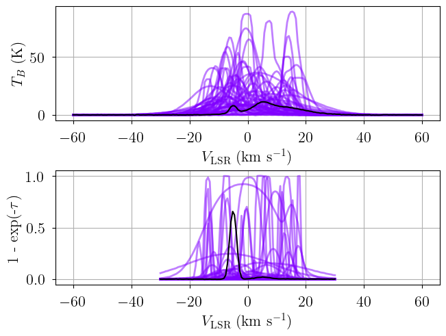
We check that our prior distributions are reasonable by drawing prior predictive checks. Each colored line is a simulated “observation” with parameters drawn from the prior distributions. You should check that these simulated observations at least somewhat overlap your actual observation (black line).
[10]:
from bayes_spec.plots import plot_predictive

# prior predictive check
prior = model.sample_prior_predictive(
    samples=1000,  # prior predictive samples
)
axes = plot_predictive(model.data, prior.prior_predictive.sel(draw=slice(None, None, 20)))
axes.ravel()[1].sharex(axes.ravel()[0])
Sampling: [TB_fwhm_norm, absorption, baseline_absorption_norm, baseline_emission_norm, emission, filling_factor, fwhm2_norm, log10_nHI_norm, log10_n_alpha_norm, tkin_factor_norm, velocity_norm, wt_ff_tkin]
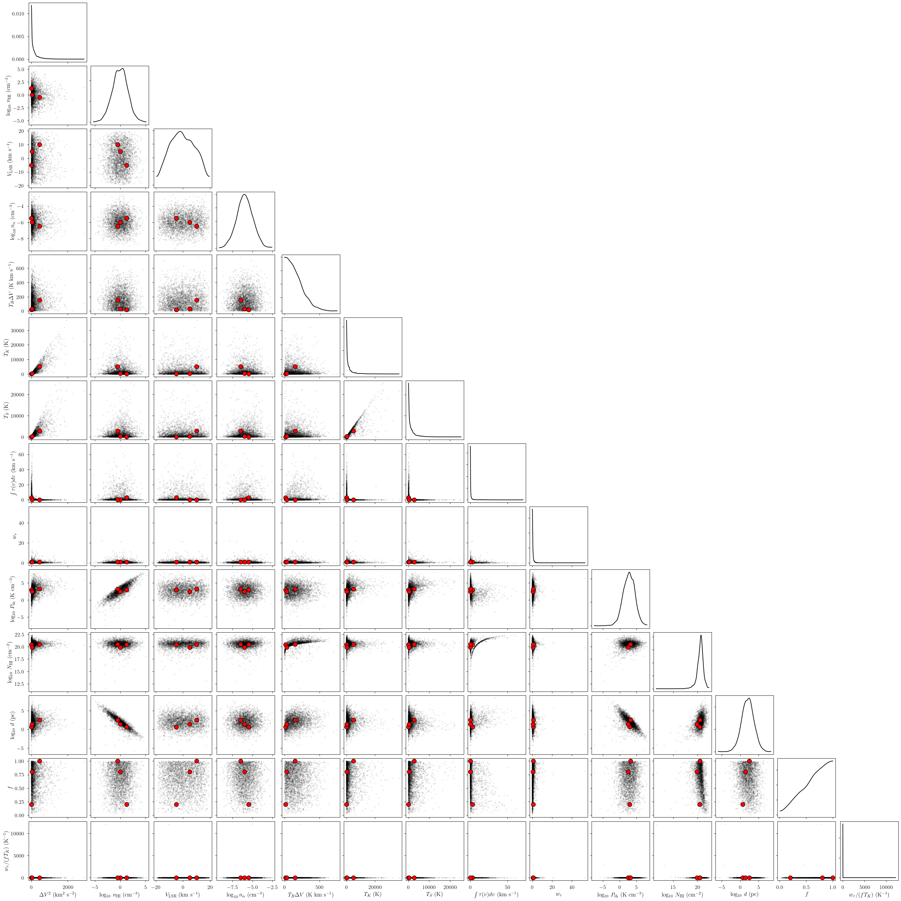
Or we can inspect the prior distributions of the derived quantities to check that they are physically reasonable. The red points represent the simulation parameters.
[11]:
print(model.cloud_freeRVs)
print(model.cloud_deterministics)
['fwhm2_norm', 'log10_nHI_norm', 'velocity_norm', 'log10_n_alpha_norm', 'TB_fwhm_norm', 'tkin_factor_norm', 'filling_factor', 'wt_ff_tkin']
['fwhm2', 'log10_nHI', 'velocity', 'log10_n_alpha', 'TB_fwhm', 'tkin', 'tspin', 'tau_total', 'absorption_weight', 'log10_Pth', 'log10_NHI', 'log10_depth']
[12]:
from bayes_spec.plots import plot_pair

var_names = model.cloud_deterministics + [p for p in model.cloud_freeRVs if "_norm" not in p]
print(var_names)
_ = plot_pair(
    prior.prior, # samples
    var_names, # var_names to plot
    combine_dims=["cloud"], # concatenate clouds
    labeller=model.labeller, # label manager
    kind="scatter", # plot type
    reference_values=sim_params, # truths
)
['fwhm2', 'log10_nHI', 'velocity', 'log10_n_alpha', 'TB_fwhm', 'tkin', 'tspin', 'tau_total', 'absorption_weight', 'log10_Pth', 'log10_NHI', 'log10_depth', 'filling_factor', 'wt_ff_tkin']
Variational Inference
We can approximate the posterior distribution using variational inference.
[13]:
start = time.time()
model.fit(
    n = 1_000_000, # maximum number of VI iterations
    draws = 1_000, # number of posterior samples
    rel_tolerance = 0.005, # VI relative convergence threshold
    abs_tolerance = 0.005, # VI absolute convergence threshold
    learning_rate = 0.001, # VI learning rate
    start = {"velocity_norm": np.linspace(0.1, 0.9, n_clouds)},
)
end = time.time()
print(f"Runtime: {(end-start)/60.0:.2f} minutes")
Convergence achieved at 53400
Interrupted at 53,399 [5%]: Average Loss = 3.0195e+05
Adding log-likelihood to trace
Runtime: 1.06 minutes
[14]:
pm.summary(model.trace.posterior)
arviz - WARNING - Shape validation failed: input_shape: (1, 1000), minimum_shape: (chains=2, draws=4)
[14]:
| mean | sd | hdi_3% | hdi_97% | mcse_mean | mcse_sd | ess_bulk | ess_tail | r_hat | |
|---|---|---|---|---|---|---|---|---|---|
| baseline_emission_norm[0] | -0.253 | 0.070 | -0.375 | -0.112 | 0.002 | 0.002 | 939.0 | 886.0 | NaN |
| baseline_absorption_norm[0] | 0.172 | 0.104 | -0.022 | 0.358 | 0.003 | 0.002 | 1000.0 | 785.0 | NaN |
| log10_nHI_norm[0] | 0.202 | 0.960 | -1.736 | 1.798 | 0.032 | 0.022 | 875.0 | 901.0 | NaN |
| log10_nHI_norm[1] | -2.525 | 0.023 | -2.566 | -2.479 | 0.001 | 0.001 | 973.0 | 945.0 | NaN |
| log10_nHI_norm[2] | 0.549 | 0.730 | -0.965 | 1.837 | 0.024 | 0.016 | 945.0 | 937.0 | NaN |
| log10_n_alpha_norm[0] | 0.389 | 0.641 | -0.736 | 1.649 | 0.021 | 0.014 | 937.0 | 1072.0 | NaN |
| log10_n_alpha_norm[1] | -3.295 | 0.001 | -3.296 | -3.294 | 0.000 | 0.000 | 809.0 | 1036.0 | NaN |
| log10_n_alpha_norm[2] | 0.668 | 0.659 | -0.628 | 1.815 | 0.021 | 0.013 | 963.0 | 979.0 | NaN |
| fwhm2_norm[0] | 0.156 | 0.003 | 0.152 | 0.162 | 0.000 | 0.000 | 947.0 | 935.0 | NaN |
| fwhm2_norm[1] | 0.026 | 0.000 | 0.026 | 0.026 | 0.000 | 0.000 | 944.0 | 823.0 | NaN |
| fwhm2_norm[2] | 2.226 | 0.014 | 2.200 | 2.254 | 0.000 | 0.000 | 985.0 | 767.0 | NaN |
| velocity_norm[0] | 0.627 | 0.001 | 0.626 | 0.629 | 0.000 | 0.000 | 829.0 | 783.0 | NaN |
| velocity_norm[1] | 0.375 | 0.000 | 0.375 | 0.375 | 0.000 | 0.000 | 963.0 | 868.0 | NaN |
| velocity_norm[2] | 0.743 | 0.001 | 0.742 | 0.745 | 0.000 | 0.000 | 997.0 | 1022.0 | NaN |
| TB_fwhm_norm[0] | 0.141 | 0.001 | 0.139 | 0.143 | 0.000 | 0.000 | 812.0 | 965.0 | NaN |
| TB_fwhm_norm[1] | 0.097 | 0.000 | 0.097 | 0.097 | 0.000 | 0.000 | 1010.0 | 951.0 | NaN |
| TB_fwhm_norm[2] | 0.774 | 0.002 | 0.770 | 0.777 | 0.000 | 0.000 | 942.0 | 878.0 | NaN |
| tkin_factor_norm[0] | 0.549 | 0.111 | 0.325 | 0.741 | 0.004 | 0.002 | 991.0 | 909.0 | NaN |
| tkin_factor_norm[1] | 0.964 | 0.001 | 0.962 | 0.966 | 0.000 | 0.000 | 873.0 | 911.0 | NaN |
| tkin_factor_norm[2] | 0.334 | 0.157 | 0.073 | 0.620 | 0.005 | 0.003 | 945.0 | 956.0 | NaN |
| filling_factor[0] | 0.698 | 0.207 | 0.315 | 0.993 | 0.007 | 0.005 | 974.0 | 937.0 | NaN |
| filling_factor[1] | 0.878 | 0.004 | 0.870 | 0.885 | 0.000 | 0.000 | 1041.0 | 944.0 | NaN |
| filling_factor[2] | 0.676 | 0.231 | 0.239 | 0.992 | 0.008 | 0.005 | 948.0 | 826.0 | NaN |
| wt_ff_tkin[0] | 0.004 | 0.000 | 0.003 | 0.004 | 0.000 | 0.000 | 1090.0 | 981.0 | NaN |
| wt_ff_tkin[1] | 0.024 | 0.000 | 0.024 | 0.024 | 0.000 | 0.000 | 1030.0 | 978.0 | NaN |
| wt_ff_tkin[2] | 0.000 | 0.000 | 0.000 | 0.000 | 0.000 | 0.000 | 929.0 | 976.0 | NaN |
| fwhm2[0] | 31.299 | 0.541 | 30.351 | 32.347 | 0.018 | 0.012 | 947.0 | 935.0 | NaN |
| fwhm2[1] | 5.270 | 0.006 | 5.258 | 5.281 | 0.000 | 0.000 | 944.0 | 823.0 | NaN |
| fwhm2[2] | 445.179 | 2.797 | 440.058 | 450.835 | 0.089 | 0.069 | 985.0 | 767.0 | NaN |
| log10_nHI[0] | 0.302 | 1.441 | -2.605 | 2.698 | 0.049 | 0.033 | 875.0 | 901.0 | NaN |
| log10_nHI[1] | -3.787 | 0.035 | -3.849 | -3.718 | 0.001 | 0.001 | 973.0 | 945.0 | NaN |
| log10_nHI[2] | 0.824 | 1.096 | -1.448 | 2.756 | 0.036 | 0.023 | 945.0 | 937.0 | NaN |
| velocity[0] | 5.100 | 0.025 | 5.052 | 5.148 | 0.001 | 0.001 | 829.0 | 783.0 | NaN |
| velocity[1] | -5.002 | 0.001 | -5.005 | -4.999 | 0.000 | 0.000 | 963.0 | 868.0 | NaN |
| velocity[2] | 9.724 | 0.034 | 9.663 | 9.793 | 0.001 | 0.001 | 997.0 | 1022.0 | NaN |
| log10_n_alpha[0] | -5.611 | 0.641 | -6.736 | -4.351 | 0.021 | 0.014 | 937.0 | 1072.0 | NaN |
| log10_n_alpha[1] | -9.295 | 0.001 | -9.296 | -9.294 | 0.000 | 0.000 | 809.0 | 1036.0 | NaN |
| log10_n_alpha[2] | -5.332 | 0.659 | -6.628 | -4.185 | 0.021 | 0.013 | 963.0 | 979.0 | NaN |
| TB_fwhm[0] | 28.243 | 0.212 | 27.866 | 28.663 | 0.007 | 0.005 | 812.0 | 965.0 | NaN |
| TB_fwhm[1] | 19.418 | 0.019 | 19.382 | 19.452 | 0.001 | 0.000 | 1010.0 | 951.0 | NaN |
| TB_fwhm[2] | 154.726 | 0.415 | 153.992 | 155.481 | 0.014 | 0.009 | 942.0 | 878.0 | NaN |
| tkin[0] | 377.744 | 75.955 | 229.925 | 513.559 | 2.378 | 1.631 | 1017.0 | 919.0 | NaN |
| tkin[1] | 111.288 | 0.177 | 110.977 | 111.627 | 0.006 | 0.004 | 910.0 | 880.0 | NaN |
| tkin[2] | 3253.986 | 1523.913 | 719.562 | 6033.750 | 49.610 | 33.422 | 941.0 | 919.0 | NaN |
| tspin[0] | 374.911 | 74.828 | 236.967 | 516.922 | 2.360 | 1.636 | 1001.0 | 874.0 | NaN |
| tspin[1] | 25.911 | 0.036 | 25.842 | 25.978 | 0.001 | 0.001 | 1006.0 | 983.0 | NaN |
| tspin[2] | 3114.891 | 1431.307 | 826.523 | 5811.709 | 46.694 | 32.735 | 940.0 | 962.0 | NaN |
| tau_total[0] | 0.145 | 0.112 | 0.061 | 0.283 | 0.004 | 0.014 | 970.0 | 1017.0 | NaN |
| tau_total[1] | 1.137 | 0.007 | 1.123 | 1.149 | 0.000 | 0.000 | 981.0 | 862.0 | NaN |
| tau_total[2] | 0.131 | 0.153 | 0.024 | 0.313 | 0.005 | 0.016 | 932.0 | 900.0 | NaN |
| absorption_weight[0] | 0.927 | 0.337 | 0.331 | 1.596 | 0.011 | 0.007 | 980.0 | 1017.0 | NaN |
| absorption_weight[1] | 2.385 | 0.012 | 2.361 | 2.407 | 0.000 | 0.000 | 1034.0 | 1016.0 | NaN |
| absorption_weight[2] | 0.726 | 0.436 | 0.041 | 1.525 | 0.014 | 0.011 | 924.0 | 908.0 | NaN |
| log10_Pth[0] | 2.870 | 1.441 | 0.012 | 5.402 | 0.049 | 0.033 | 865.0 | 901.0 | NaN |
| log10_Pth[1] | -1.741 | 0.035 | -1.804 | -1.673 | 0.001 | 0.001 | 970.0 | 945.0 | NaN |
| log10_Pth[2] | 4.283 | 1.115 | 2.033 | 6.235 | 0.036 | 0.024 | 972.0 | 871.0 | NaN |
| log10_NHI[0] | 19.927 | 0.174 | 19.740 | 20.251 | 0.006 | 0.007 | 990.0 | 937.0 | NaN |
| log10_NHI[1] | 19.730 | 0.003 | 19.725 | 19.735 | 0.000 | 0.000 | 1024.0 | 907.0 | NaN |
| log10_NHI[2] | 20.687 | 0.209 | 20.480 | 21.099 | 0.007 | 0.009 | 946.0 | 826.0 | NaN |
| log10_depth[0] | 1.135 | 1.449 | -1.365 | 3.987 | 0.049 | 0.033 | 867.0 | 850.0 | NaN |
| log10_depth[1] | 5.028 | 0.035 | 4.959 | 5.089 | 0.001 | 0.001 | 952.0 | 937.0 | NaN |
| log10_depth[2] | 1.374 | 1.120 | -0.853 | 3.471 | 0.037 | 0.024 | 912.0 | 865.0 | NaN |
[15]:
posterior = model.sample_posterior_predictive(
    thin=10,  # keep one in {thin} posterior samples
)
axes = plot_predictive(model.data, posterior.posterior_predictive)
axes.ravel()[1].sharex(axes.ravel()[0])
Sampling: [absorption, emission]

Posterior Sampling: MCMC
We can sample from the posterior distribution using MCMC. We increase target_accept because this model has some degeneracies.
[16]:
start = time.time()
model.sample(
    init="advi+adapt_diag",  # initialization strategy
    tune=1000,  # tuning samples
    draws=1000,  # posterior samples
    chains=8,  # number of independent chains
    cores=8,  # number of parallel chains
    init_kwargs={
        "rel_tolerance": 0.005,
        "abs_tolerance": 0.005,
        "learning_rate": 0.001,
        "start": {"velocity_norm": np.linspace(0.1, 0.9, n_clouds)},
    },  # VI initialization arguments
    nuts_kwargs={"target_accept": 0.9},  # NUTS arguments
)
end = time.time()
print(f"Runtime: {(end-start)/60.0:.2f} minutes")
Initializing NUTS using custom advi+adapt_diag strategy
Convergence achieved at 53400
Interrupted at 53,399 [5%]: Average Loss = 3.0195e+05
Multiprocess sampling (8 chains in 8 jobs)
NUTS: [baseline_emission_norm, baseline_absorption_norm, fwhm2_norm, log10_nHI_norm, velocity_norm, log10_n_alpha_norm, TB_fwhm_norm, tkin_factor_norm, filling_factor, wt_ff_tkin]
Sampling 8 chains for 1_000 tune and 1_000 draw iterations (8_000 + 8_000 draws total) took 350 seconds.
Adding log-likelihood to trace
There were 136 divergences in converged chains.
Runtime: 7.22 minutes
[17]:
model.solve(
    init_params="random_from_data", # GMM initialization strategy
    n_init=10, # number of GMM initilizations
    max_iter=1_000, # maximum number of GMM iterations
    kl_div_threshold=0.1, # covergence threshold
)
GMM converged to unique solution
Check that the effective sample sizes are large and the covergence statistic r_hat is close to 1! If not, you may have to increase the number of tuning steps (tune=2000) or the NUTS acceptance rate (target_accept=0.9).
[18]:
print("solutions:", model.solutions)
az.summary(model.trace["solution_0"])
# this also works: az.summary(model.trace.solution_0)
solutions: [0]
[18]:
| mean | sd | hdi_3% | hdi_97% | mcse_mean | mcse_sd | ess_bulk | ess_tail | r_hat | |
|---|---|---|---|---|---|---|---|---|---|
| baseline_emission_norm[0] | -0.234 | 0.092 | -0.408 | -0.061 | 0.002 | 0.001 | 3105.0 | 4297.0 | 1.00 |
| baseline_absorption_norm[0] | 0.172 | 0.148 | -0.107 | 0.454 | 0.002 | 0.002 | 4444.0 | 4414.0 | 1.00 |
| log10_nHI_norm[0] | 0.004 | 1.001 | -1.750 | 1.989 | 0.020 | 0.011 | 2591.0 | 4311.0 | 1.00 |
| log10_nHI_norm[1] | -0.002 | 1.007 | -1.797 | 1.964 | 0.015 | 0.012 | 4435.0 | 4228.0 | 1.00 |
| log10_nHI_norm[2] | -0.074 | 0.981 | -1.861 | 1.793 | 0.020 | 0.011 | 2428.0 | 4434.0 | 1.00 |
| log10_n_alpha_norm[0] | -0.013 | 1.009 | -1.881 | 1.862 | 0.028 | 0.017 | 1333.0 | 1164.0 | 1.01 |
| log10_n_alpha_norm[1] | 0.001 | 1.009 | -1.854 | 1.962 | 0.016 | 0.011 | 4019.0 | 4748.0 | 1.00 |
| log10_n_alpha_norm[2] | -0.060 | 0.957 | -1.789 | 1.791 | 0.019 | 0.010 | 2406.0 | 4808.0 | 1.00 |
| fwhm2_norm[0] | 0.161 | 0.005 | 0.152 | 0.171 | 0.000 | 0.000 | 2028.0 | 2756.0 | 1.00 |
| fwhm2_norm[1] | 0.026 | 0.000 | 0.026 | 0.026 | 0.000 | 0.000 | 4155.0 | 4852.0 | 1.00 |
| fwhm2_norm[2] | 2.195 | 0.023 | 2.151 | 2.237 | 0.000 | 0.000 | 2728.0 | 4441.0 | 1.00 |
| velocity_norm[0] | 0.627 | 0.001 | 0.626 | 0.628 | 0.000 | 0.000 | 2791.0 | 3841.0 | 1.00 |
| velocity_norm[1] | 0.375 | 0.000 | 0.375 | 0.375 | 0.000 | 0.000 | 5145.0 | 5413.0 | 1.00 |
| velocity_norm[2] | 0.746 | 0.001 | 0.743 | 0.749 | 0.000 | 0.000 | 2016.0 | 4059.0 | 1.00 |
| TB_fwhm_norm[0] | 0.148 | 0.005 | 0.139 | 0.158 | 0.000 | 0.000 | 1108.0 | 809.0 | 1.01 |
| TB_fwhm_norm[1] | 0.097 | 0.008 | 0.083 | 0.113 | 0.000 | 0.000 | 739.0 | 1554.0 | 1.02 |
| TB_fwhm_norm[2] | 0.764 | 0.005 | 0.754 | 0.774 | 0.000 | 0.000 | 1765.0 | 3306.0 | 1.00 |
| tkin_factor_norm[0] | 0.434 | 0.212 | 0.097 | 0.833 | 0.006 | 0.003 | 1073.0 | 818.0 | 1.00 |
| tkin_factor_norm[1] | 0.154 | 0.091 | 0.044 | 0.315 | 0.004 | 0.004 | 731.0 | 1351.0 | 1.02 |
| tkin_factor_norm[2] | 0.453 | 0.213 | 0.099 | 0.854 | 0.004 | 0.002 | 3272.0 | 3858.0 | 1.00 |
| filling_factor[0] | 0.669 | 0.231 | 0.261 | 1.000 | 0.004 | 0.002 | 3333.0 | 3019.0 | 1.00 |
| filling_factor[1] | 0.577 | 0.199 | 0.250 | 0.967 | 0.007 | 0.003 | 723.0 | 1407.0 | 1.02 |
| filling_factor[2] | 0.671 | 0.235 | 0.243 | 1.000 | 0.003 | 0.002 | 4633.0 | 3316.0 | 1.00 |
| wt_ff_tkin[0] | 0.003 | 0.000 | 0.003 | 0.004 | 0.000 | 0.000 | 624.0 | 333.0 | 1.02 |
| wt_ff_tkin[1] | 0.080 | 0.008 | 0.066 | 0.094 | 0.000 | 0.000 | 882.0 | 1692.0 | 1.01 |
| wt_ff_tkin[2] | 0.000 | 0.000 | 0.000 | 0.000 | 0.000 | 0.000 | 1561.0 | 1298.0 | 1.01 |
| fwhm2[0] | 32.188 | 1.038 | 30.349 | 34.284 | 0.023 | 0.013 | 2028.0 | 2756.0 | 1.00 |
| fwhm2[1] | 5.266 | 0.013 | 5.242 | 5.291 | 0.000 | 0.000 | 4155.0 | 4852.0 | 1.00 |
| fwhm2[2] | 439.012 | 4.592 | 430.204 | 447.420 | 0.088 | 0.052 | 2728.0 | 4441.0 | 1.00 |
| log10_nHI[0] | 0.006 | 1.502 | -2.625 | 2.983 | 0.030 | 0.016 | 2591.0 | 4311.0 | 1.00 |
| log10_nHI[1] | -0.004 | 1.511 | -2.695 | 2.946 | 0.023 | 0.018 | 4435.0 | 4228.0 | 1.00 |
| log10_nHI[2] | -0.110 | 1.471 | -2.792 | 2.690 | 0.030 | 0.016 | 2428.0 | 4434.0 | 1.00 |
| velocity[0] | 5.076 | 0.029 | 5.024 | 5.132 | 0.001 | 0.000 | 2791.0 | 3841.0 | 1.00 |
| velocity[1] | -5.001 | 0.001 | -5.003 | -4.998 | 0.000 | 0.000 | 5145.0 | 5413.0 | 1.00 |
| velocity[2] | 9.837 | 0.060 | 9.726 | 9.950 | 0.001 | 0.001 | 2016.0 | 4059.0 | 1.00 |
| log10_n_alpha[0] | -6.013 | 1.009 | -7.881 | -4.138 | 0.028 | 0.017 | 1333.0 | 1164.0 | 1.01 |
| log10_n_alpha[1] | -5.999 | 1.009 | -7.854 | -4.038 | 0.016 | 0.011 | 4019.0 | 4748.0 | 1.00 |
| log10_n_alpha[2] | -6.060 | 0.957 | -7.789 | -4.209 | 0.019 | 0.010 | 2406.0 | 4808.0 | 1.00 |
| TB_fwhm[0] | 29.631 | 1.077 | 27.858 | 31.605 | 0.040 | 0.059 | 1108.0 | 809.0 | 1.01 |
| TB_fwhm[1] | 19.469 | 1.680 | 16.543 | 22.580 | 0.061 | 0.024 | 739.0 | 1554.0 | 1.02 |
| TB_fwhm[2] | 152.833 | 1.040 | 150.854 | 154.827 | 0.025 | 0.015 | 1765.0 | 3306.0 | 1.00 |
| tkin[0] | 309.585 | 150.276 | 56.278 | 576.770 | 4.071 | 1.771 | 1098.0 | 811.0 | 1.00 |
| tkin[1] | 24.983 | 9.251 | 14.790 | 41.329 | 0.365 | 0.425 | 733.0 | 1370.0 | 1.02 |
| tkin[2] | 4352.617 | 2049.009 | 922.855 | 8166.648 | 35.636 | 18.975 | 3267.0 | 3856.0 | 1.00 |
| tspin[0] | 301.464 | 144.863 | 55.614 | 557.850 | 3.802 | 1.663 | 1149.0 | 815.0 | 1.00 |
| tspin[1] | 24.946 | 9.215 | 14.834 | 41.290 | 0.348 | 0.420 | 732.0 | 1373.0 | 1.02 |
| tspin[2] | 3254.774 | 1744.473 | 399.499 | 6409.431 | 32.124 | 18.229 | 2687.0 | 3298.0 | 1.00 |
| tau_total[0] | 0.269 | 0.260 | 0.047 | 0.719 | 0.008 | 0.013 | 1397.0 | 1521.0 | 1.00 |
| tau_total[1] | 2.674 | 0.257 | 2.180 | 3.146 | 0.003 | 0.003 | 6137.0 | 5240.0 | 1.00 |
| tau_total[2] | 0.142 | 0.192 | 0.020 | 0.380 | 0.004 | 0.019 | 3263.0 | 4129.0 | 1.00 |
| absorption_weight[0] | 0.691 | 0.442 | 0.051 | 1.507 | 0.010 | 0.005 | 1400.0 | 1410.0 | 1.00 |
| absorption_weight[1] | 1.023 | 0.101 | 0.846 | 1.219 | 0.001 | 0.001 | 6111.0 | 5318.0 | 1.00 |
| absorption_weight[2] | 0.748 | 0.511 | 0.043 | 1.725 | 0.008 | 0.006 | 3271.0 | 4169.0 | 1.00 |
| log10_Pth[0] | 2.436 | 1.523 | -0.408 | 5.303 | 0.030 | 0.017 | 2535.0 | 3980.0 | 1.00 |
| log10_Pth[1] | 1.372 | 1.513 | -1.432 | 4.228 | 0.023 | 0.018 | 4366.0 | 4884.0 | 1.00 |
| log10_Pth[2] | 3.467 | 1.471 | 0.806 | 6.342 | 0.028 | 0.017 | 2683.0 | 4907.0 | 1.00 |
| log10_NHI[0] | 19.980 | 0.202 | 19.742 | 20.359 | 0.003 | 0.004 | 3820.0 | 3413.0 | 1.00 |
| log10_NHI[1] | 20.060 | 0.137 | 19.841 | 20.315 | 0.005 | 0.003 | 787.0 | 1469.0 | 1.01 |
| log10_NHI[2] | 20.687 | 0.213 | 20.468 | 21.091 | 0.003 | 0.005 | 4708.0 | 3382.0 | 1.00 |
| log10_depth[0] | 1.485 | 1.510 | -1.392 | 4.247 | 0.030 | 0.016 | 2535.0 | 4475.0 | 1.00 |
| log10_depth[1] | 1.575 | 1.520 | -1.386 | 4.317 | 0.023 | 0.018 | 4331.0 | 4159.0 | 1.00 |
| log10_depth[2] | 2.308 | 1.489 | -0.548 | 5.034 | 0.030 | 0.017 | 2478.0 | 4579.0 | 1.00 |
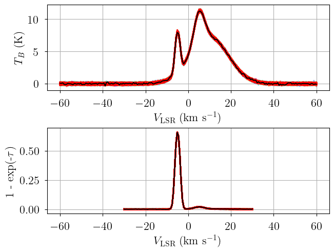
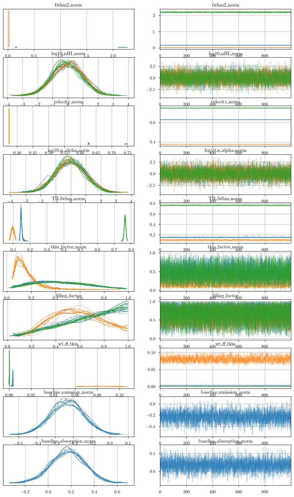
We generate posterior predictive checks as well as a trace plot of the individual chains. In the posterior predictive plot, we show each chain as a different color. Each line is one posterior sample.
[19]:
posterior = model.sample_posterior_predictive(
    thin=10,  # keep one in {thin} posterior samples
)
axes = plot_predictive(model.data, posterior.posterior_predictive)
axes.ravel()[0].sharex(axes.ravel()[1])
Sampling: [absorption, emission]
[20]:
from bayes_spec.plots import plot_traces

_ = plot_traces(model.trace.posterior, model.cloud_freeRVs + model.baseline_freeRVs + model.hyper_freeRVs)
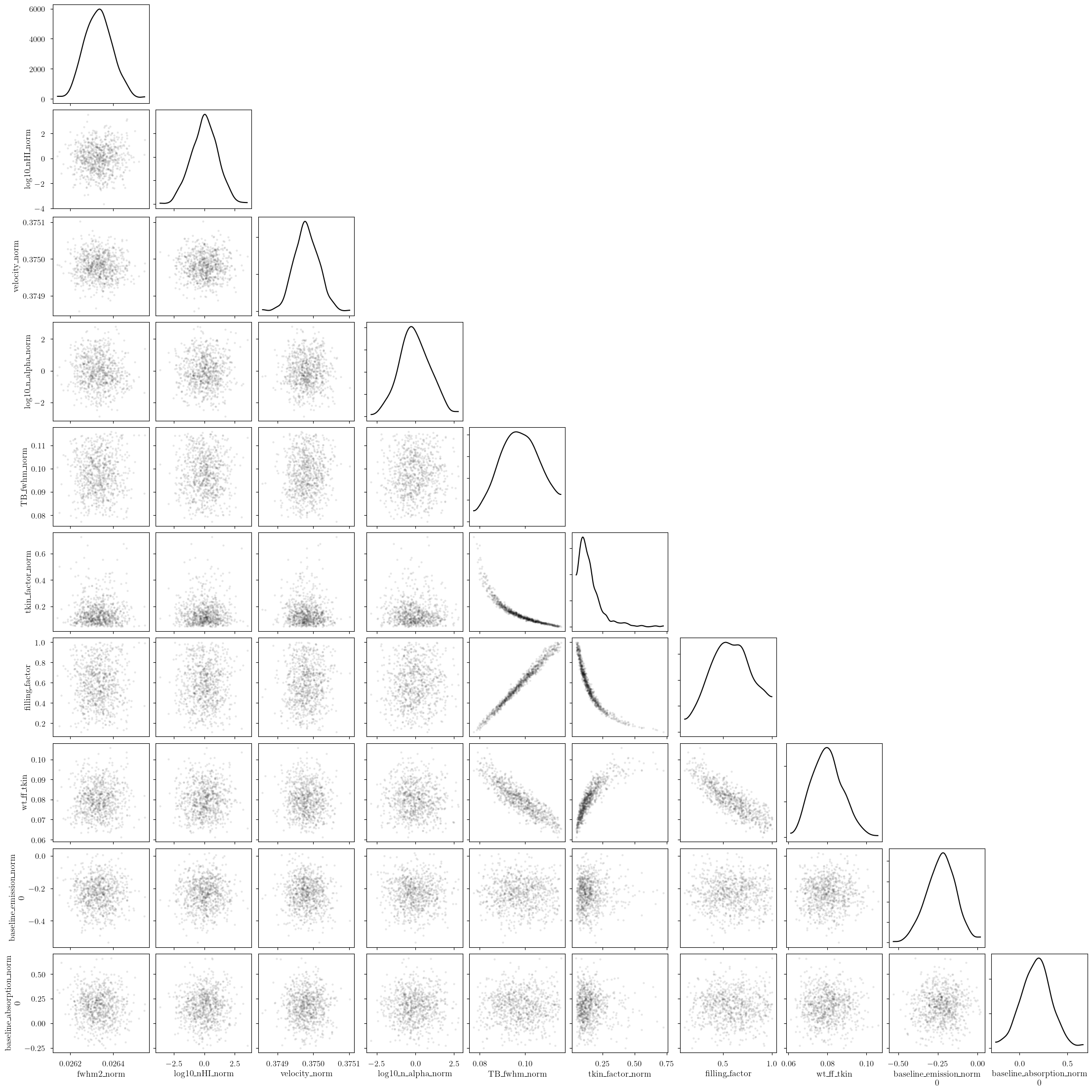
We can inspect the posterior distribution pair plots. First, the free parameters for all clouds. Keep an eye out for any strong degeneracies or non-linear correlations. If present, then these features can cause the posterior sampling to be inefficient. It may be worth re-parameterizing your model to remove these effects. Alternatively, increasing tune and target_accept can help.
[21]:
_ = plot_pair(
    model.trace.solution_0.sel(draw=slice(None, None, 10)), # samples
    model.cloud_freeRVs, # var_names to plot
    combine_dims=["cloud"], # concatenate clouds
    kind="scatter", # plot type
)
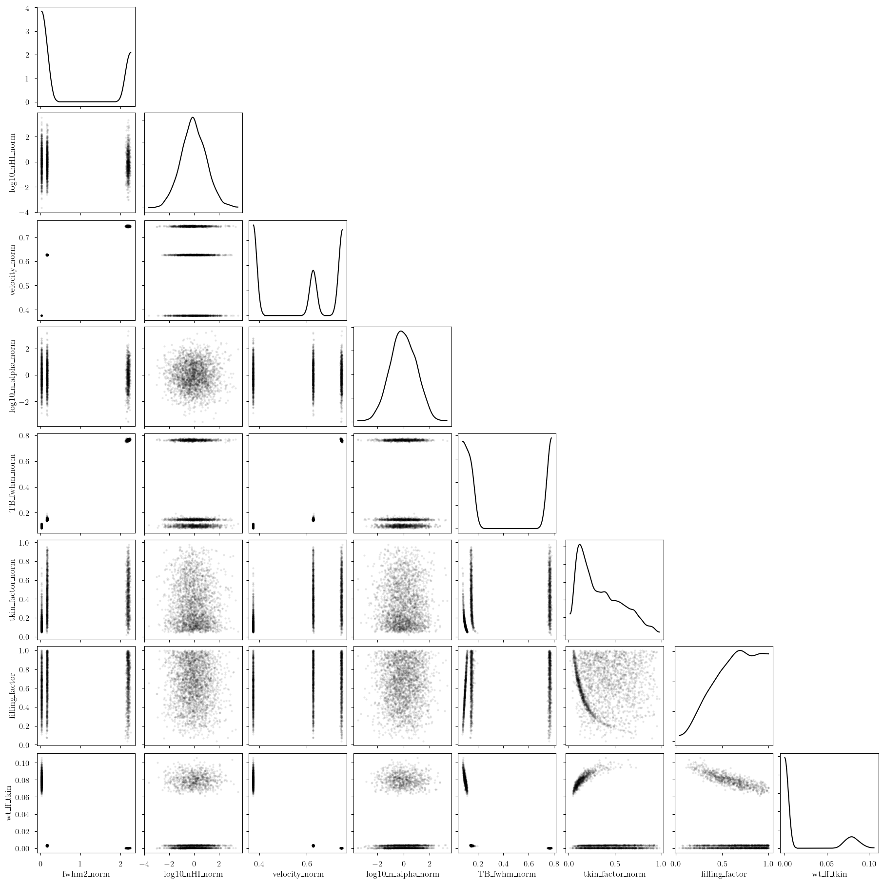
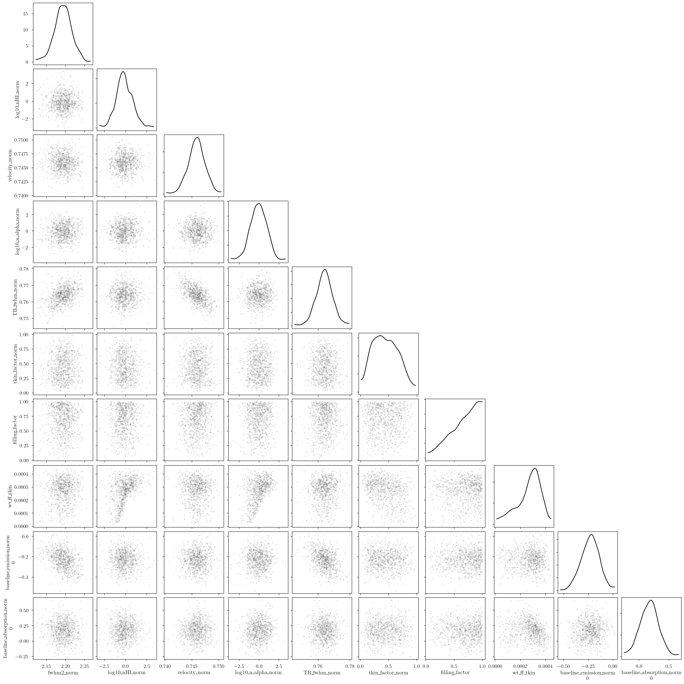
Notice that there are three posterior modes. These correspond to the three clouds of the model.
[22]:
_ = plot_pair(
    model.trace.solution_0.sel(draw=slice(None, None, 10)), # samples
    ["velocity", "fwhm2"], # var_names to plot
    combine_dims=None, # do not concatenate clouds
    kind="scatter", # plot type
)
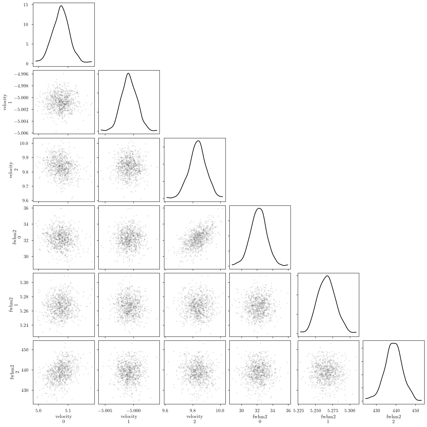
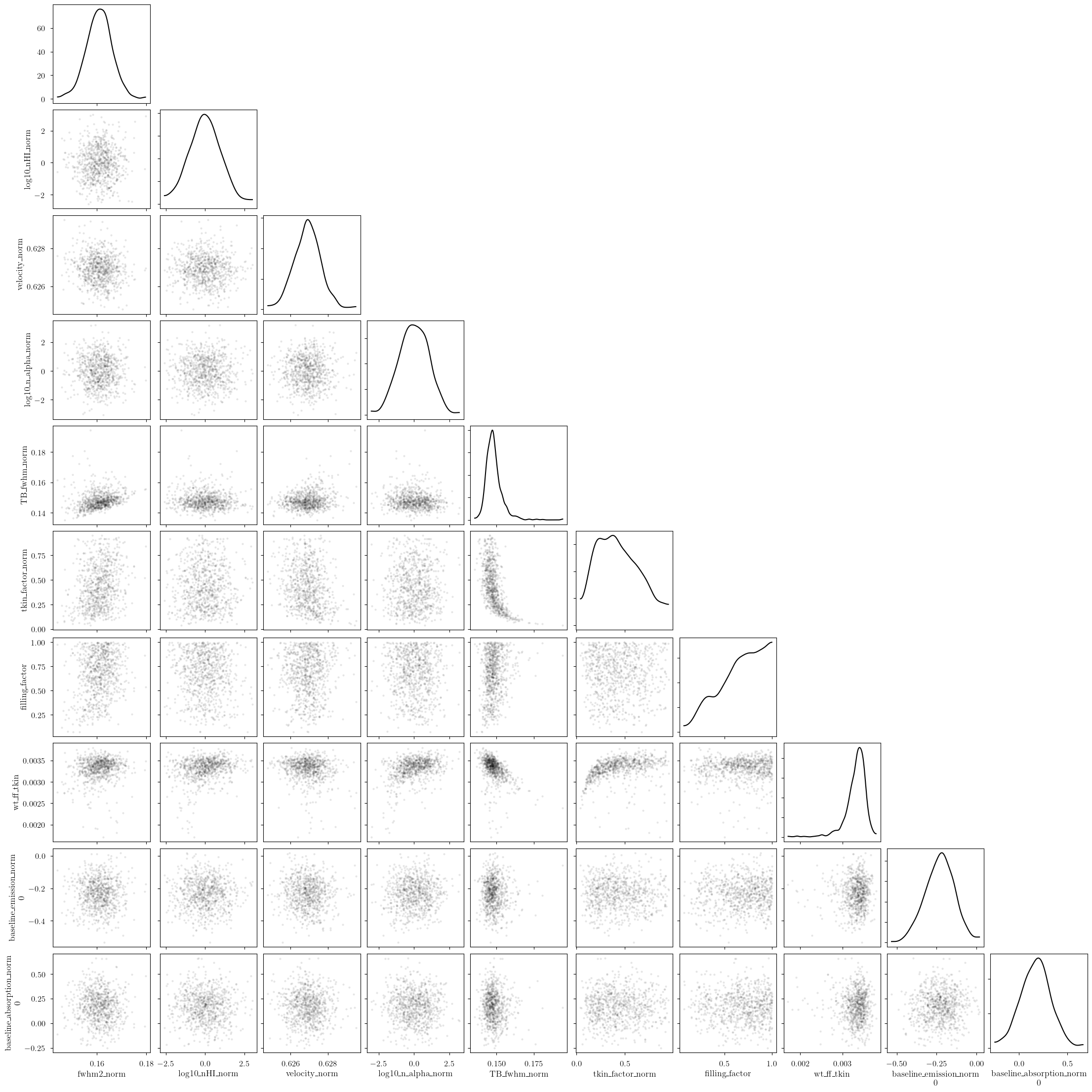
We can plot the posterior distributions of the deterministic quantities for a single cloud.
[23]:
_ = plot_pair(
    model.trace.solution_0.sel(cloud=0, draw=slice(None, None, 10)), # samples
    model.cloud_freeRVs + model.hyper_freeRVs + model.baseline_freeRVs, # var_names to plot
    kind="scatter", # plot type
)
[24]:
_ = plot_pair(
    model.trace.solution_0.sel(cloud=1, draw=slice(None, None, 10)), # samples
    model.cloud_freeRVs + model.hyper_freeRVs + model.baseline_freeRVs, # var_names to plot
    kind="scatter", # plot type
)
[25]:
_ = plot_pair(
    model.trace.solution_0.sel(cloud=2, draw=slice(None, None, 10)), # samples
    model.cloud_freeRVs + model.hyper_freeRVs + model.baseline_freeRVs, # var_names to plot
    kind="scatter", # plot type
)
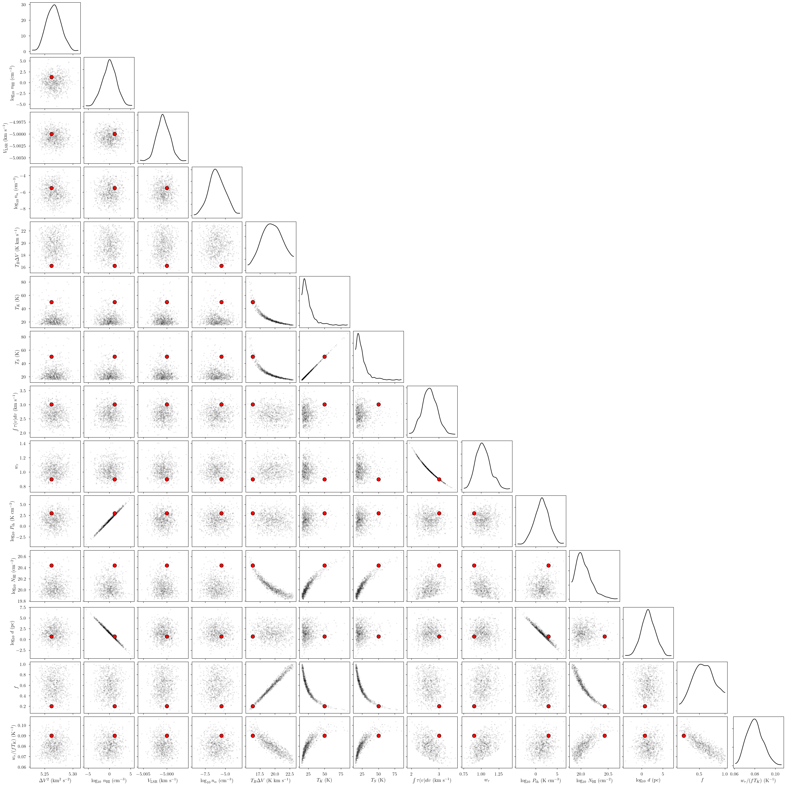
And the deterministic quantities. The red points represent the simulation parameters.
[26]:
_ = plot_pair(
    model.trace.solution_0.sel(draw=slice(None, None, 10)), # samples
    var_names, # var_names to plot
    combine_dims=["cloud"], # concatenate clouds
    labeller=model.labeller, # label manager
    kind="scatter", # plot type
    reference_values=sim_params, # truths
)
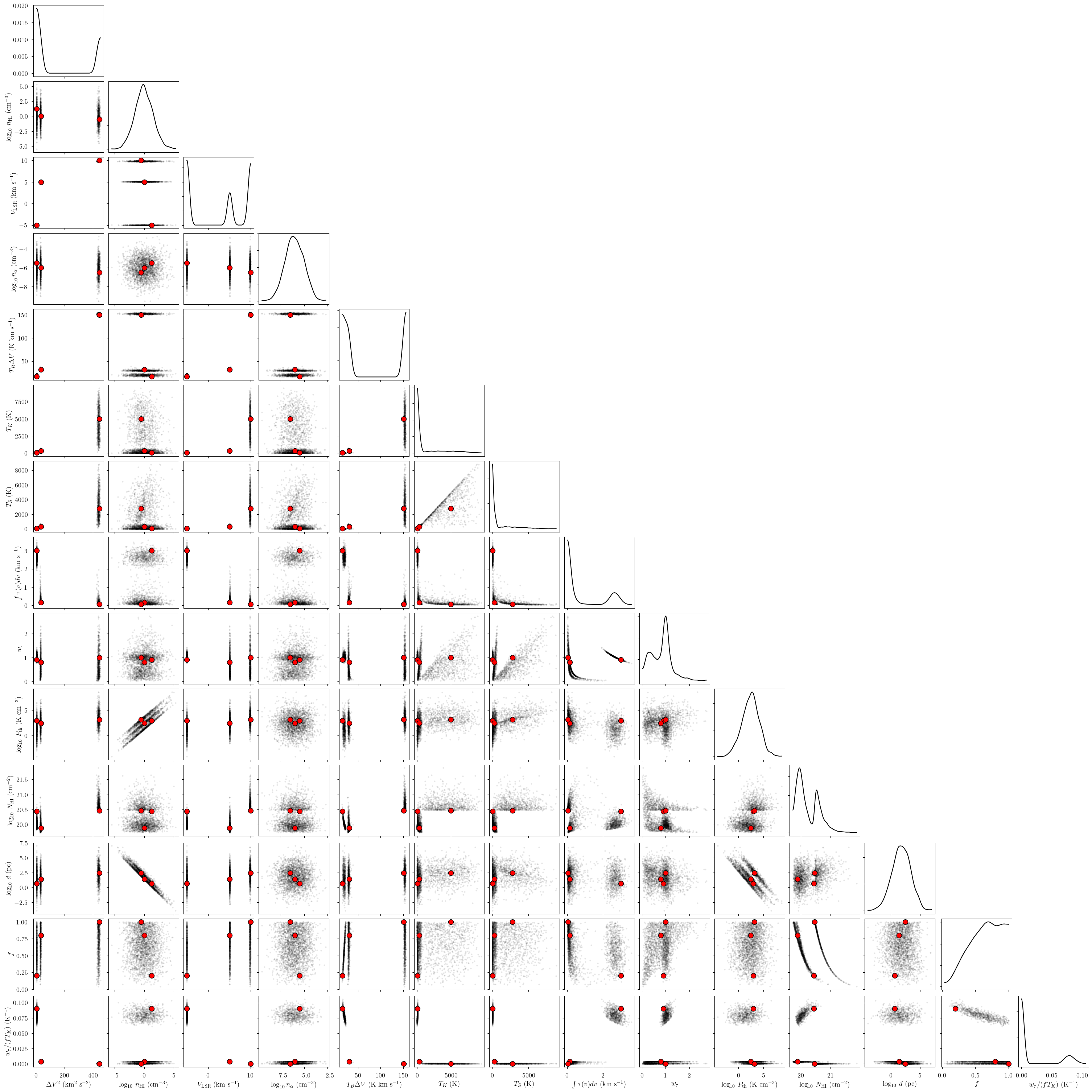
Notice that there are three posterior modes. These correspond to the three clouds of the model. We can plot the posterior distributions of the deterministic quantities for a single cloud.
[27]:
# identify simulation cloud corresponding to each posterior cloud
sim_cloud_map = {}
for i in range(n_clouds):
    posterior_velocity = model.trace.solution_0['velocity'].sel(cloud=i).data.mean()
    match = np.argmin(np.abs(sim_params["velocity"] - posterior_velocity))
    sim_cloud_map[i] = match
sim_cloud_map
[27]:
{0: np.int64(1), 1: np.int64(0), 2: np.int64(2)}
[28]:
print("cloud freeRVs", model.cloud_freeRVs)
print("cloud deterministics", model.cloud_deterministics)
print("hyper freeRVs", model.hyper_freeRVs)
print("hyper deterministics", model.hyper_deterministics)
cloud freeRVs ['fwhm2_norm', 'log10_nHI_norm', 'velocity_norm', 'log10_n_alpha_norm', 'TB_fwhm_norm', 'tkin_factor_norm', 'filling_factor', 'wt_ff_tkin']
cloud deterministics ['fwhm2', 'log10_nHI', 'velocity', 'log10_n_alpha', 'TB_fwhm', 'tkin', 'tspin', 'tau_total', 'absorption_weight', 'log10_Pth', 'log10_NHI', 'log10_depth']
hyper freeRVs []
hyper deterministics []
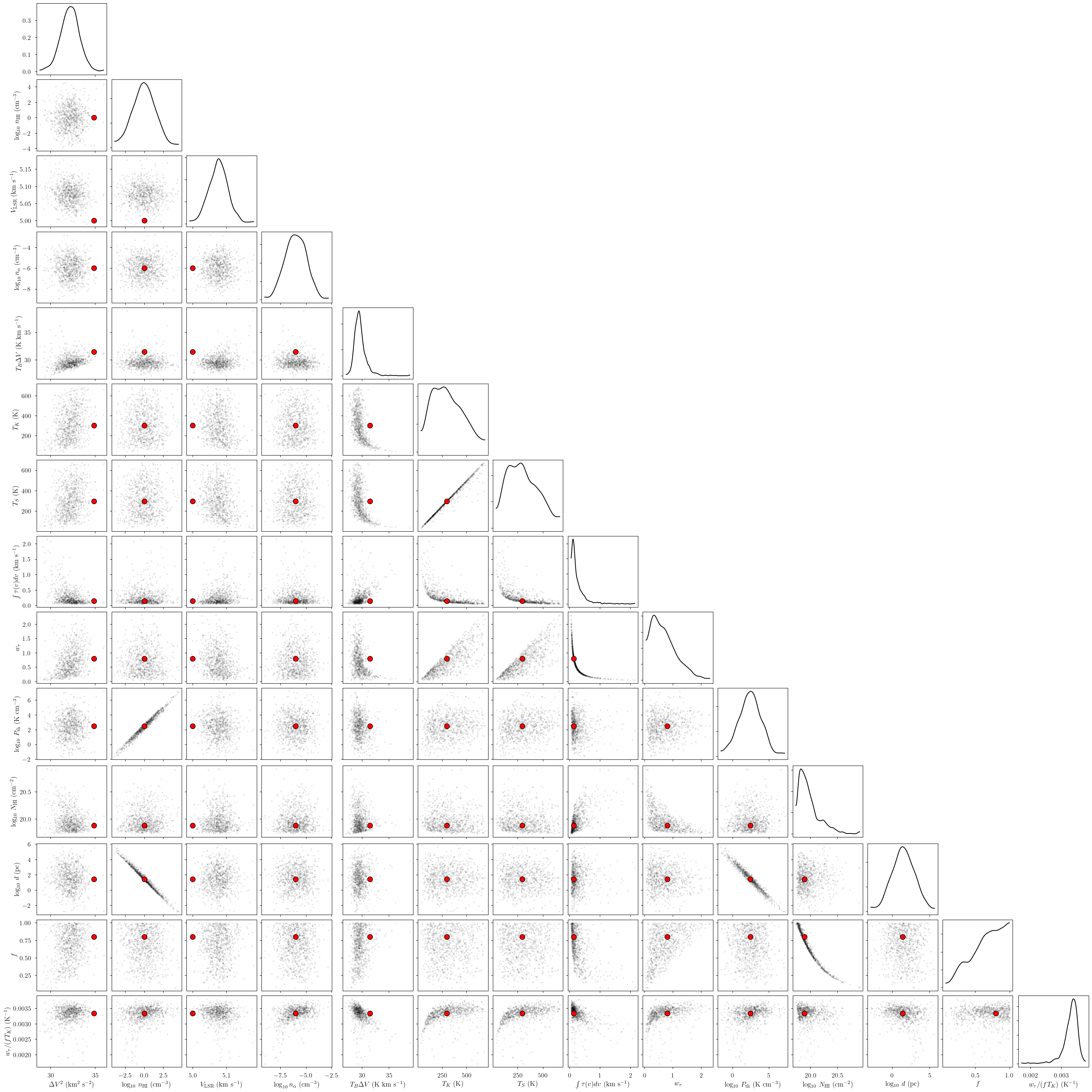
[29]:
cloud = 0

# subset of sim_params
my_sim_params = {}
for var_name in var_names:
    my_sim_params[var_name] = sim_params[var_name][sim_cloud_map[cloud]]

_ = plot_pair(
    model.trace.solution_0.sel(cloud=cloud, draw=slice(None, None, 10)), # samples
    var_names, # var_names to plot
    labeller=model.labeller, # label manager
    kind="scatter", # plot type
    reference_values=my_sim_params, # truths
)
[30]:
cloud = 1

# subset of sim_params
my_sim_params = {}
for var_name in var_names:
    my_sim_params[var_name] = sim_params[var_name][sim_cloud_map[cloud]]

_ = plot_pair(
    model.trace.solution_0.sel(cloud=cloud, draw=slice(None, None, 10)), # samples
    var_names, # var_names to plot
    labeller=model.labeller, # label manager
    kind="scatter", # plot type
    reference_values=my_sim_params, # truths
)
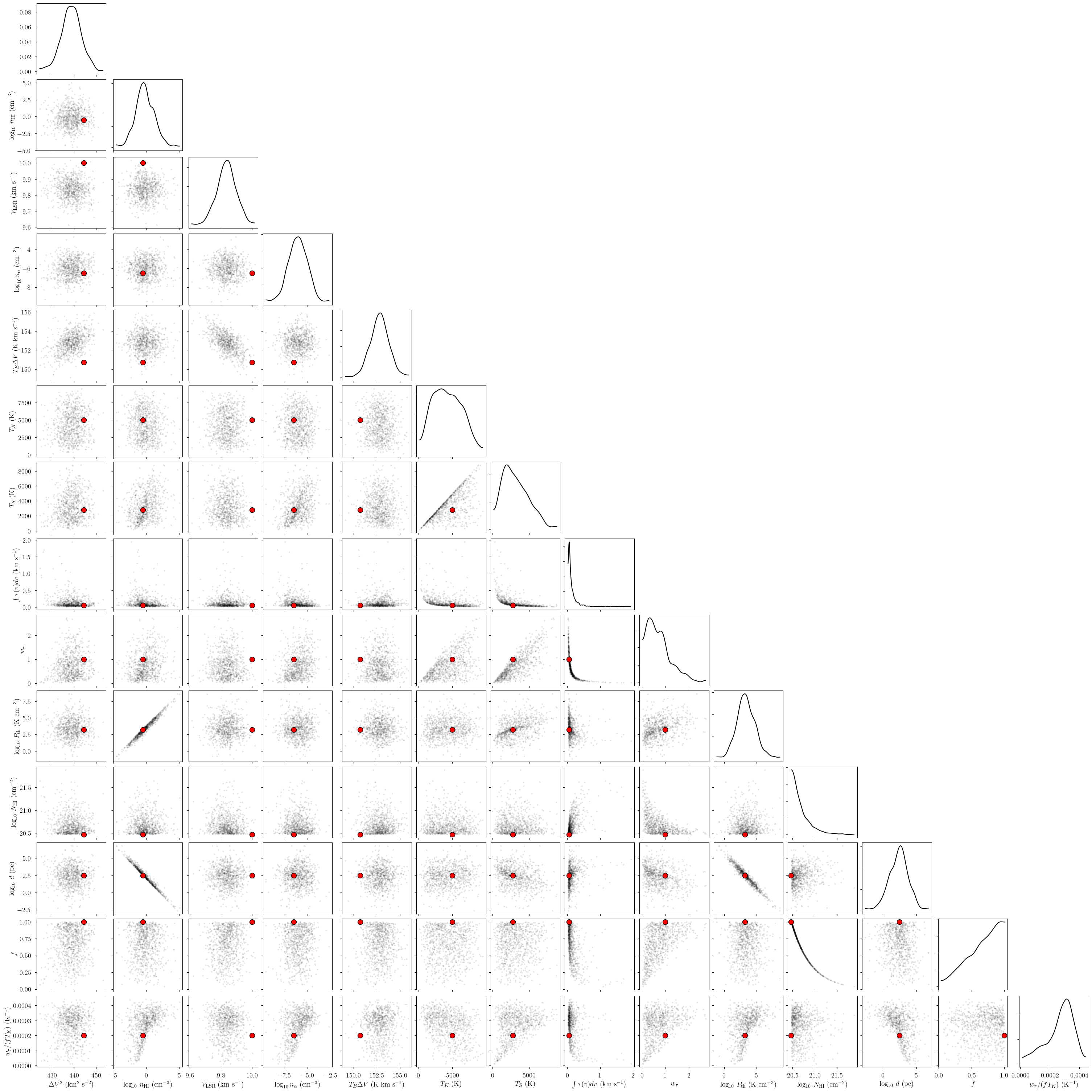
[31]:
cloud = 2

# subset of sim_params
my_sim_params = {}
for var_name in var_names:
    my_sim_params[var_name] = sim_params[var_name][sim_cloud_map[cloud]]

_ = plot_pair(
    model.trace.solution_0.sel(cloud=cloud, draw=slice(None, None, 10)), # samples
    var_names, # var_names to plot
    labeller=model.labeller, # label manager
    kind="scatter", # plot type
    reference_values=my_sim_params, # truths
)
Finally, we can get the posterior statistics, Bayesian Information Criterion (BIC), etc.
[32]:
point_stats = az.summary(model.trace.solution_0, kind="stats", hdi_prob=0.68)
print("BIC:", model.bic())
display(point_stats)
BIC: -1322.9379586390694
| mean | sd | hdi_16% | hdi_84% | |
|---|---|---|---|---|
| baseline_emission_norm[0] | -0.234 | 0.092 | -0.322 | -0.141 |
| baseline_absorption_norm[0] | 0.172 | 0.148 | 0.016 | 0.309 |
| log10_nHI_norm[0] | 0.004 | 1.001 | -0.969 | 1.032 |
| log10_nHI_norm[1] | -0.002 | 1.007 | -1.025 | 0.960 |
| log10_nHI_norm[2] | -0.074 | 0.981 | -1.147 | 0.761 |
| log10_n_alpha_norm[0] | -0.013 | 1.009 | -0.938 | 1.074 |
| log10_n_alpha_norm[1] | 0.001 | 1.009 | -1.012 | 0.978 |
| log10_n_alpha_norm[2] | -0.060 | 0.957 | -1.049 | 0.832 |
| fwhm2_norm[0] | 0.161 | 0.005 | 0.156 | 0.166 |
| fwhm2_norm[1] | 0.026 | 0.000 | 0.026 | 0.026 |
| fwhm2_norm[2] | 2.195 | 0.023 | 2.173 | 2.218 |
| velocity_norm[0] | 0.627 | 0.001 | 0.626 | 0.628 |
| velocity_norm[1] | 0.375 | 0.000 | 0.375 | 0.375 |
| velocity_norm[2] | 0.746 | 0.001 | 0.744 | 0.747 |
| TB_fwhm_norm[0] | 0.148 | 0.005 | 0.143 | 0.151 |
| TB_fwhm_norm[1] | 0.097 | 0.008 | 0.088 | 0.105 |
| TB_fwhm_norm[2] | 0.764 | 0.005 | 0.759 | 0.769 |
| tkin_factor_norm[0] | 0.434 | 0.212 | 0.158 | 0.599 |
| tkin_factor_norm[1] | 0.154 | 0.091 | 0.054 | 0.172 |
| tkin_factor_norm[2] | 0.453 | 0.213 | 0.162 | 0.620 |
| filling_factor[0] | 0.669 | 0.231 | 0.564 | 1.000 |
| filling_factor[1] | 0.577 | 0.199 | 0.328 | 0.754 |
| filling_factor[2] | 0.671 | 0.235 | 0.576 | 1.000 |
| wt_ff_tkin[0] | 0.003 | 0.000 | 0.003 | 0.004 |
| wt_ff_tkin[1] | 0.080 | 0.008 | 0.070 | 0.086 |
| wt_ff_tkin[2] | 0.000 | 0.000 | 0.000 | 0.000 |
| fwhm2[0] | 32.188 | 1.038 | 31.184 | 33.200 |
| fwhm2[1] | 5.266 | 0.013 | 5.253 | 5.279 |
| fwhm2[2] | 439.012 | 4.592 | 434.568 | 443.582 |
| log10_nHI[0] | 0.006 | 1.502 | -1.453 | 1.548 |
| log10_nHI[1] | -0.004 | 1.511 | -1.538 | 1.440 |
| log10_nHI[2] | -0.110 | 1.471 | -1.721 | 1.142 |
| velocity[0] | 5.076 | 0.029 | 5.046 | 5.103 |
| velocity[1] | -5.001 | 0.001 | -5.002 | -5.000 |
| velocity[2] | 9.837 | 0.060 | 9.777 | 9.895 |
| log10_n_alpha[0] | -6.013 | 1.009 | -6.938 | -4.926 |
| log10_n_alpha[1] | -5.999 | 1.009 | -7.012 | -5.022 |
| log10_n_alpha[2] | -6.060 | 0.957 | -7.049 | -5.168 |
| TB_fwhm[0] | 29.631 | 1.077 | 28.543 | 30.230 |
| TB_fwhm[1] | 19.469 | 1.680 | 17.503 | 21.100 |
| TB_fwhm[2] | 152.833 | 1.040 | 151.827 | 153.854 |
| tkin[0] | 309.585 | 150.276 | 108.635 | 419.805 |
| tkin[1] | 24.983 | 9.251 | 15.469 | 26.431 |
| tkin[2] | 4352.617 | 2049.009 | 1549.440 | 5951.917 |
| tspin[0] | 301.464 | 144.863 | 104.366 | 404.395 |
| tspin[1] | 24.946 | 9.215 | 15.473 | 26.403 |
| tspin[2] | 3254.774 | 1744.473 | 971.164 | 4375.793 |
| tau_total[0] | 0.269 | 0.260 | 0.053 | 0.271 |
| tau_total[1] | 2.674 | 0.257 | 2.403 | 2.906 |
| tau_total[2] | 0.142 | 0.192 | 0.025 | 0.132 |
| absorption_weight[0] | 0.691 | 0.442 | 0.092 | 0.869 |
| absorption_weight[1] | 1.023 | 0.101 | 0.909 | 1.100 |
| absorption_weight[2] | 0.748 | 0.511 | 0.103 | 0.948 |
| log10_Pth[0] | 2.436 | 1.523 | 0.921 | 3.964 |
| log10_Pth[1] | 1.372 | 1.513 | -0.066 | 2.912 |
| log10_Pth[2] | 3.467 | 1.471 | 1.922 | 4.788 |
| log10_NHI[0] | 19.980 | 0.202 | 19.759 | 20.031 |
| log10_NHI[1] | 20.060 | 0.137 | 19.882 | 20.130 |
| log10_NHI[2] | 20.687 | 0.213 | 20.471 | 20.713 |
| log10_depth[0] | 1.485 | 1.510 | 0.103 | 3.127 |
| log10_depth[1] | 1.575 | 1.520 | 0.046 | 3.027 |
| log10_depth[2] | 2.308 | 1.489 | 0.992 | 3.895 |
[ ]: