Optimization Tutorial
Trey V. Wenger (c) July 2025
Here we demonstrate how to optimize the number of cloud components in a EmissionAbsorptionPhysicalModel model.
[1]:
# General imports
import time

import matplotlib.pyplot as plt
import arviz as az
import pandas as pd
import numpy as np
import pymc as pm

print("pymc version:", pm.__version__)
print("arviz version:", az.__version__)

import bayes_spec
print("bayes_spec version:", bayes_spec.__version__)

import caribou_hi
print("caribou_hi version:", caribou_hi.__version__)

# Notebook configuration
pd.options.display.max_rows = None
pymc version: 5.22.0
arviz version: 0.22.0dev
bayes_spec version: 1.9.0
caribou_hi version: 4.1.0+3.g94a913e.dirty
Model Definition and Simulated Data
[2]:
from bayes_spec import SpecData
# spectral axes definitions
emission_axis = np.linspace(-60.0, 60.0, 200) # km s-1
absorption_axis = np.linspace(-30.0, 30.0, 100) # km s-1
# data noise can either be a scalar (assumed constant noise across the spectrum)
# or an array of the same length as the data
rms_emission = 0.1 # K
rms_absorption = 0.001 # 1 - exp(-tau)
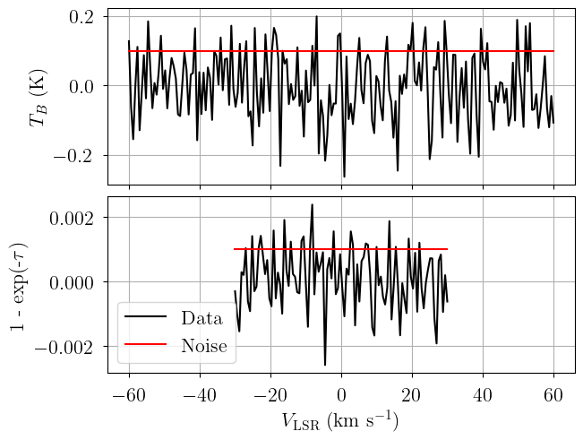
# brightness data. In this case, we just throw in some random data for now
# since we are only doing this in order to simulate some actual data.
emission = rms_emission * np.random.randn(len(emission_axis))
absorption = rms_absorption * np.random.randn(len(absorption_axis))
dummy_data = {
"emission": SpecData(
emission_axis,
emission,
rms_emission,
xlabel=r"$V_{\rm LSR}$ (km s$^{-1}$)",
ylabel=r"$T_B$ (K)",
),
"absorption": SpecData(
absorption_axis,
absorption,
rms_absorption,
xlabel=r"$V_{\rm LSR}$ (km s$^{-1}$)",
ylabel=r"1 - exp(-$\tau$)",
),
}
# Plot dummy data
fig, axes = plt.subplots(2, layout="constrained", sharex=True)
axes[0].plot(dummy_data["emission"].spectral, dummy_data["emission"].brightness, "k-")
axes[0].plot(dummy_data["emission"].spectral, dummy_data["emission"].noise, "r-")
axes[1].plot(dummy_data["absorption"].spectral, dummy_data["absorption"].brightness, "k-", label="Data")
axes[1].plot(dummy_data["absorption"].spectral, dummy_data["absorption"].noise, "r-", label="Noise")
axes[1].set_xlabel(dummy_data["emission"].xlabel)
axes[0].set_ylabel(dummy_data["emission"].ylabel)
axes[1].set_ylabel(dummy_data["absorption"].ylabel)
_ = axes[1].legend(loc="lower left")
[3]:
from caribou_hi import EmissionAbsorptionPhysicalModel

# Initialize and define the model
n_clouds = 3
baseline_degree = 0
model = EmissionAbsorptionPhysicalModel(
    dummy_data,
    n_clouds=n_clouds,
    baseline_degree=baseline_degree,
    bg_temp = 3.77, # assumed background temperature (K)
    seed=1234,
    verbose=True
)
model.add_priors(
    prior_filling_factor=[2.0, 1.0],  # filling factor prior shape
    prior_ff_NHI=1.0e21,  # filling factor * column density prior width (cm-2)
    prior_fwhm2_thermal_fraction=[2.0, 2.0], # thermal FWHM^2 fraction prior shape
    prior_sigma_log10_NHI=0.5, # log-normal column density distribution width
    prior_fwhm2=200.0, # FWHM^2 prior width (km2 s-2)
    prior_velocity=[-15.0, 15.0],  # lower and upper limit of velocity prior (km/s)
    prior_log10_n_alpha=[-6.0, 1.0],  # log10(n_alpha) prior width (cm-3)
    prior_nth_fwhm_1pc=[1.75, 0.25], # non-thermal FWHM at 1 pc prior mean and width (km s-1)
    prior_depth_nth_fwhm_power=[0.3, 0.1], # non-thermal FWHM vs. depth power prior mean and width
    prior_fwhm_L=None, # Assume Gaussian line profile
    prior_baseline_coeffs=None, # Default baseline priors
)
model.add_likelihood()
[4]:
from caribou_hi import physics
# Simulation parameters
filling_factor = np.array([0.2, 0.8, 1.0])
absorption_weight = np.array([0.9, 0.8, 1.0])
log10_nHI = np.array([1.25, 0.0, -0.5])
tkin = np.array([50.0, 300.0, 5000.0])
n_alpha = np.array([1.0e-6, 2.0e-6, 3.0e-6])
depth = np.array([5.0, 25.0, 300.0])
nth_fwhm_1pc = np.array([2.0, 1.75, 1.5])
depth_nth_fwhm_power = np.array([0.2, 0.3, 0.4])
tspin = physics.calc_spin_temp(tkin, 10.0**log10_nHI, n_alpha).eval()
print("tspin", tspin)
fwhm2_nonthermal = physics.calc_nonthermal_fwhm(depth, nth_fwhm_1pc, depth_nth_fwhm_power)**2.0
print("fwhm2_nonthermal", fwhm2_nonthermal)
fwhm2_thermal = physics.calc_thermal_fwhm2(tkin)
print("fwhm2_thermal", fwhm2_thermal)
fwhm2 = fwhm2_nonthermal + fwhm2_thermal
print("fwhm2", fwhm2)
fwhm2_thermal_fraction = fwhm2_thermal/fwhm2
print("fwhm2_thermal_fraction", fwhm2_thermal_fraction)
log10_Pth = np.log10(tkin) + log10_nHI
print("log10_Pth", log10_Pth)
log10_NHI = log10_nHI + np.log10(depth) + 18.489351
print("log10_NHI", log10_NHI)
tau_total = physics.calc_tau_total(10.0**log10_NHI, tspin)
print("tau_total", tau_total)
#wt_ff_tspin = absorption_weight / filling_factor / tspin
#print("wt_ff_tspin", wt_ff_tspin)
wt_ff_fwhm2_thermal = absorption_weight / filling_factor / fwhm2_thermal
print("wt_ff_fwhm2_thermal", wt_ff_fwhm2_thermal)
sim_params = {
"wt_ff_fwhm2_thermal": wt_ff_fwhm2_thermal,
"absorption_weight": absorption_weight,
"filling_factor": filling_factor,
"log10_NHI": log10_NHI,
"tau_total": tau_total,
"tspin": tspin,
"fwhm2": fwhm2,
"fwhm2_thermal_fraction": fwhm2_thermal_fraction,
"velocity": np.array([-5.0, 5.0, 10.0]),
"n_alpha": n_alpha,
"nth_fwhm_1pc": nth_fwhm_1pc,
"depth_nth_fwhm_power": depth_nth_fwhm_power,
"baseline_emission_norm": [0.0],
"baseline_absorption_norm": [0.0],
}
# add derived quantities to sim_params
for key in model.cloud_deterministics:
if key not in sim_params.keys():
sim_params[key] = model.model[key].eval(sim_params, on_unused_input="ignore")
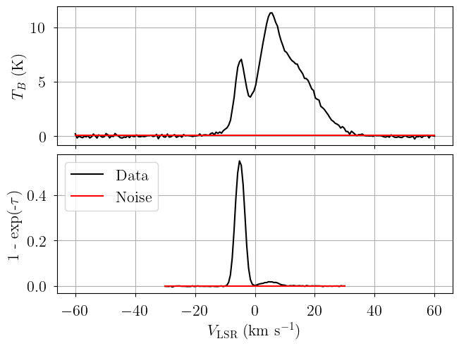
# Evaluate and save simulated observation
emission = model.model["emission"].eval(sim_params, on_unused_input="ignore")
absorption = model.model["absorption"].eval(sim_params, on_unused_input="ignore")
data = {
"emission": SpecData(
emission_axis,
emission,
rms_emission,
xlabel=r"$V_{\rm LSR}$ (km s$^{-1}$)",
ylabel=r"$T_B$ (K)",
),
"absorption": SpecData(
absorption_axis,
absorption,
rms_absorption,
xlabel=r"$V_{\rm LSR}$ (km s$^{-1}$)",
ylabel=r"1 - exp(-$\tau$)",
),
}
tspin [  49.97911226  298.78900835 4259.26982821]
fwhm2_nonthermal [  7.61461575  21.12711044 215.71459099]
fwhm2_thermal [  2.2876605  13.725963  228.76605  ]
fwhm2 [  9.90227625  34.85307344 444.48064099]
fwhm2_thermal_fraction [0.2310237 0.3938236 0.5146817]
log10_Pth [2.94897    2.47712125 3.19897   ]
log10_NHI [20.438321   19.88729101 20.46647225]
tau_total [3.01218479 0.14166923 0.03771258]
wt_ff_fwhm2_thermal [1.9670751  0.07285463 0.00437128]
[5]:
sim_params
[5]:
{'wt_ff_fwhm2_thermal': array([1.9670751 , 0.07285463, 0.00437128]),
 'absorption_weight': array([0.9, 0.8, 1. ]),
 'filling_factor': array([0.2, 0.8, 1. ]),
 'log10_NHI': array([20.438321  , 19.88729101, 20.46647225]),
 'tau_total': array([3.01218479, 0.14166923, 0.03771258]),
 'tspin': array([  49.97911226,  298.78900835, 4259.26982821]),
 'fwhm2': array([  9.90227625,  34.85307344, 444.48064099]),
 'fwhm2_thermal_fraction': array([0.2310237, 0.3938236, 0.5146817]),
 'velocity': array([-5.,  5., 10.]),
 'n_alpha': array([1.e-06, 2.e-06, 3.e-06]),
 'nth_fwhm_1pc': array([2.  , 1.75, 1.5 ]),
 'depth_nth_fwhm_power': array([0.2, 0.3, 0.4]),
 'baseline_emission_norm': [0.0],
 'baseline_absorption_norm': [0.0],
 'log10_n_alpha': array([-5.75395025, -6.4990086 , -5.89087838]),
 'fwhm2_thermal': array([  2.2876605,  13.725963 , 228.76605  ]),
 'tkin': array([  50.,  300., 5000.]),
 'fwhm2_nonthermal': array([  7.61461575,  21.12711044, 215.71459099]),
 'log10_depth': array([0.69897   , 1.39794001, 2.47712125]),
 'log10_nHI': array([ 1.25,  0.  , -0.5 ]),
 'log10_Pth': array([2.94897   , 2.47712125, 3.19897   ]),
 'log10_Pnth': array([4.95888799, 4.1520801 , 4.66111952]),
 'log10_Ptot': array([4.96311227, 4.16116407, 4.67585106])}
[6]:
# Plot data
fig, axes = plt.subplots(2, layout="constrained", sharex=True)
axes[0].plot(data["emission"].spectral, data["emission"].brightness, "k-")
axes[0].plot(data["emission"].spectral, data["emission"].noise, "r-")
axes[1].plot(data["absorption"].spectral, data["absorption"].brightness, "k-", label="Data")
axes[1].plot(data["absorption"].spectral, data["absorption"].noise, "r-", label="Noise")
axes[1].set_xlabel(data["emission"].xlabel)
axes[0].set_ylabel(data["emission"].ylabel)
axes[1].set_ylabel(data["absorption"].ylabel)
_ = axes[1].legend(loc="upper left")
Optimize
We use the Optimize class for optimization.
[7]:
from bayes_spec import Optimize

# Initialize optimizer
opt = Optimize(
    EmissionAbsorptionPhysicalModel,  # model definition
    data,  # data dictionary
    max_n_clouds=5,  # maximum number of clouds
    baseline_degree=baseline_degree,  # polynomial baseline degree
    bg_temp=3.77,  # assumed background brightness temperature (K)
    seed=1234,  # random seed
    verbose=True,  # verbosity
)

# Define each model
opt.add_priors(
    prior_filling_factor=[2.0, 1.0],  # filling factor prior shape
    prior_ff_NHI=1.0e21,  # filling factor * column density prior width (cm-2)
    prior_fwhm2_thermal_fraction=[2.0, 2.0], # thermal FWHM^2 fraction prior shape
    prior_sigma_log10_NHI=0.5, # log-normal column density distribution width
    prior_fwhm2=200.0, # FWHM^2 prior width (km2 s-2)
    prior_velocity=[-15.0, 15.0],  # lower and upper limit of velocity prior (km/s)
    prior_log10_n_alpha=[-6.0, 1.0],  # log10(n_alpha) prior width (cm-3)
    prior_nth_fwhm_1pc=[1.75, 0.25], # non-thermal FWHM at 1 pc prior mean and width (km s-1)
    prior_depth_nth_fwhm_power=[0.3, 0.1], # non-thermal FWHM vs. depth power prior mean and width
    prior_fwhm_L=None, # Assume Gaussian line profile
    prior_baseline_coeffs=None, # Default baseline priors
)
opt.add_likelihood()
Optimize has created max_n_clouds models, where opt.models[1] has n_clouds=1, opt.models[2] has n_clouds=2, etc.
[8]:
print(opt.models[4])
print(opt.models[4].n_clouds)
<caribou_hi.emission_absorption_physical_model.EmissionAbsorptionPhysicalModel object at 0x716ae0200c30>
4
By default (approx=True), the optimization algorithm first loops over every model and approximates the posterior distribution using variational inference. This is generally a bad idea, since VI is only an approximation and tends to struggle with complex models. Instead we use approx=False to sample every model with MCMC. This is slower but more robust.
We can supply arguments to fit and sample via dictionaries. Whichever model is the first to have a BIC within bic_threshold of the minimum BIC is the “best” model. The algorithm will terminate early if successive models have increasing BICs or fail to converge.
[9]:
fit_kwargs = {
    "rel_tolerance": 0.005,
    "abs_tolerance": 0.005,
    "learning_rate": 0.001,
}
sample_kwargs = {
    "chains": 8,
    "cores": 8,
    "n_init": 200_000,
    "init_kwargs": fit_kwargs,
    "nuts_kwargs": {"target_accept": 0.9},
}
solve_kwargs = {
    "init_params": "random_from_data",
    "n_init": 10,
    "max_iter": 1_000,
    "kl_div_threshold": 0.1,
}
opt.optimize(
    bic_threshold=10.0,
    sample_kwargs=sample_kwargs,
    fit_kwargs=fit_kwargs,
    solve_kwargs=solve_kwargs,
    approx=False,
    start_spread = {"velocity_norm": [0.1, 0.9]},
)
Null hypothesis BIC = 1.433e+06
Sampling n_cloud = 1 posterior...
Initializing NUTS using custom advi+adapt_diag strategy
Convergence achieved at 46600
Interrupted at 46,599 [23%]: Average Loss = 5.0785e+05
Multiprocess sampling (8 chains in 8 jobs)
NUTS: [baseline_emission_norm, baseline_absorption_norm, fwhm2_norm, velocity_norm, log10_n_alpha_norm, nth_fwhm_1pc, depth_nth_fwhm_power, ff_NHI_norm, fwhm2_thermal_fraction, filling_factor, wt_ff_tkin]
Sampling 8 chains for 1_000 tune and 1_000 draw iterations (8_000 + 8_000 draws total) took 157 seconds.
Adding log-likelihood to trace
GMM converged to unique solution
n_cloud = 1 solution = 0 BIC = 1.680e+05

Sampling n_cloud = 2 posterior...
Initializing NUTS using custom advi+adapt_diag strategy
Convergence achieved at 85200
Interrupted at 85,199 [42%]: Average Loss = 2.7226e+05
Multiprocess sampling (8 chains in 8 jobs)
NUTS: [baseline_emission_norm, baseline_absorption_norm, fwhm2_norm, velocity_norm, log10_n_alpha_norm, nth_fwhm_1pc, depth_nth_fwhm_power, ff_NHI_norm, fwhm2_thermal_fraction, filling_factor, wt_ff_tkin]
Sampling 8 chains for 1_000 tune and 1_000 draw iterations (8_000 + 8_000 draws total) took 191 seconds.
Adding log-likelihood to trace
GMM converged to unique solution
n_cloud = 2 solution = 0 BIC = 5.528e+03

Sampling n_cloud = 3 posterior...
Initializing NUTS using custom advi+adapt_diag strategy
Convergence achieved at 104000
Interrupted at 103,999 [51%]: Average Loss = 2.7689e+05
Multiprocess sampling (8 chains in 8 jobs)
NUTS: [baseline_emission_norm, baseline_absorption_norm, fwhm2_norm, velocity_norm, log10_n_alpha_norm, nth_fwhm_1pc, depth_nth_fwhm_power, ff_NHI_norm, fwhm2_thermal_fraction, filling_factor, wt_ff_tkin]
Sampling 8 chains for 1_000 tune and 1_000 draw iterations (8_000 + 8_000 draws total) took 196 seconds.
Adding log-likelihood to trace
GMM converged to unique solution
n_cloud = 3 solution = 0 BIC = -1.299e+03

Sampling n_cloud = 4 posterior...
Initializing NUTS using custom advi+adapt_diag strategy
Convergence achieved at 87300
Interrupted at 87,299 [43%]: Average Loss = 4.4508e+05
Multiprocess sampling (8 chains in 8 jobs)
NUTS: [baseline_emission_norm, baseline_absorption_norm, fwhm2_norm, velocity_norm, log10_n_alpha_norm, nth_fwhm_1pc, depth_nth_fwhm_power, ff_NHI_norm, fwhm2_thermal_fraction, filling_factor, wt_ff_tkin]
Sampling 8 chains for 1_000 tune and 1_000 draw iterations (8_000 + 8_000 draws total) took 406 seconds.
Adding log-likelihood to trace
There were 245 divergences in converged chains.
GMM converged to unique solution
5 of 8 chains appear converged.
Label order mismatch in solution 0
Chain 1 order: [1 0 2 3]
Chain 2 order: [1 0 2 3]
Chain 3 order: [1 0 3 2]
Chain 4 order: [1 0 2 3]
Chain 5 order: [1 0 2 3]
Adopting (first) most common order: [1 0 2 3]
n_cloud = 4 solution = 0 BIC = -1.247e+03

Stopping criteria met.
Sampling n_cloud = 5 posterior...
Initializing NUTS using custom advi+adapt_diag strategy
Convergence achieved at 168500
Interrupted at 168,499 [84%]: Average Loss = 3.0913e+05
Multiprocess sampling (8 chains in 8 jobs)
NUTS: [baseline_emission_norm, baseline_absorption_norm, fwhm2_norm, velocity_norm, log10_n_alpha_norm, nth_fwhm_1pc, depth_nth_fwhm_power, ff_NHI_norm, fwhm2_thermal_fraction, filling_factor, wt_ff_tkin]
Sampling 8 chains for 1_000 tune and 1_000 draw iterations (8_000 + 8_000 draws total) took 425 seconds.
Adding log-likelihood to trace
There were 277 divergences in converged chains.
No solution found!
0 of 8 chains appear converged.

Stopping criteria met.
Stopping early.
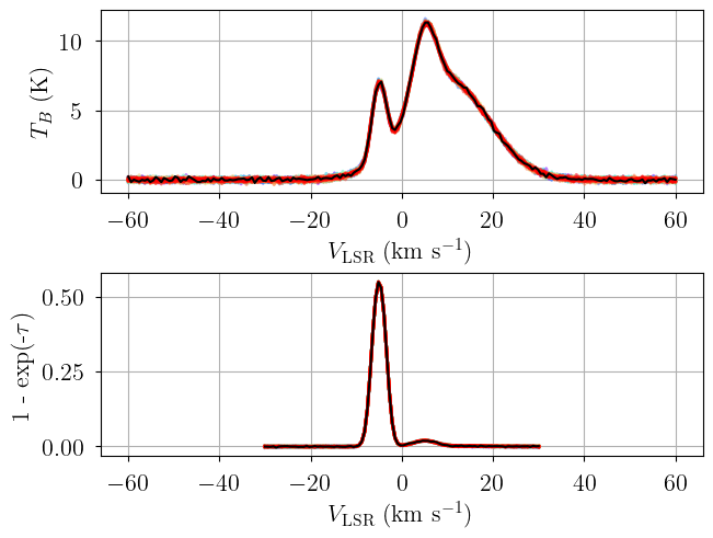
[10]:
opt.best_model.n_clouds
[10]:
3
[11]:
from bayes_spec.plots import plot_predictive

posterior = opt.best_model.sample_posterior_predictive(
    thin=100, # keep one in {thin} posterior samples
)
axes = plot_predictive(opt.best_model.data, posterior.posterior_predictive)
axes.ravel()[0].sharex(axes.ravel()[1])
Sampling: [absorption, emission]
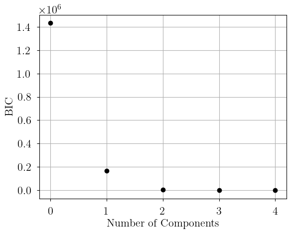
[12]:
plt.plot(opt.bics.keys(), opt.bics.values(), 'ko')
plt.xlabel("Number of Components")
plt.ylabel("BIC")
[12]:
Text(0, 0.5, 'BIC')
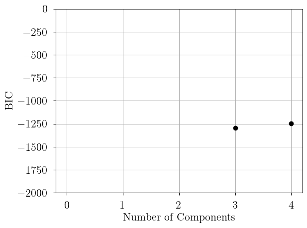
[13]:
plt.plot(opt.bics.keys(), opt.bics.values(), 'ko')
plt.xlabel("Number of Components")
plt.ylabel("BIC")
plt.ylim(-2000, 0)
[13]:
(-2000.0, 0.0)
[ ]: